Chapter 2: Binomial and Trinomial Trees

This chapter covers European and American option pricing by backward induction on a CRR binomial tree, along with Delta and Gamma estimation. It then introduces flexible binomial trees, Richardson extrapolation, binomial Black–Scholes trees, and Boyle trinomial trees. Pricing errors and convergence curves show how these methods compare in accuracy and computational effort.

Chapter setup: package imports and example parameters

The setup cell below imports the packages needed for computation and plotting, then sets the display format and example parameters.

# Common code: import the packages needed for computation and plotting
import sys
from dataclasses import replace
from pathlib import Path

import matplotlib.pyplot as plt
import numpy as np
import pandas as pd

project_root = Path.cwd()
while not (project_root / "src").exists() and project_root != project_root.parent:
    project_root = project_root.parent
sys.path.insert(0, str(project_root / "src"))

from quant_option_pricing import (
    AmericanOption,
    BlackScholesModel,
    EuropeanOption,
    TreeSettings,
)
from quant_option_pricing.black_scholes import (
    black_scholes_greeks,
    black_scholes_formula,
)
plt.style.use("seaborn-v0_8-whitegrid")
plt.rcParams["font.family"] = "DejaVu Sans"
plt.rcParams["axes.unicode_minus"] = False
plt.rcParams["figure.dpi"] = 160
plt.rcParams["savefig.dpi"] = 200
np.set_printoptions(precision=6, suppress=True)
pd.set_option("display.precision", 6)

# Model, option, and tree settings for the default examples
model = BlackScholesModel(rate=0.06, volatility=0.20)
option = EuropeanOption.put(spot=40.0, strike=45.0, maturity=0.5)
settings = TreeSettings(n_steps=100)

2.1 Cox-Ross-Rubinstein (CRR) Binomial Tree

In the BSM model, the stock price $S_t$ follows geometric Brownian motion under the risk-neutral measure:

\[ S_t=S_0\exp\left[\left(r-\frac{\sigma^2}{2}\right)t+\sigma W_t\right] \tag{2.1.1} \]

where $S_0$ denotes the current stock price, $r$ the risk-free interest rate, $\sigma$ the stock volatility, and $W_t$ Brownian motion.

Cox–Ross–Rubinstein (1979) proposed a binomial tree approximation to price options under the BSM model. The CRR construction divides the time to maturity $T$ into $n$ equal intervals, with time points $0,h,2h,\ldots,nh$, where $h=T/n$. On the binomial tree, if the underlying asset price at time $kh$ is $S_k$, the stock price at time $(k+1)h$ can take only two values: with probability $p$, it rises to $uS_k$; with probability $1-p$, it falls to $dS_k$, where $u>e^{rh}>d>0$. The resulting binomial tree is shown in Figure 2.1.

This binomial tree is called a recombining tree. Recombination limits the growth in the number of nodes: an upward move followed by a downward move reaches the same node as a downward move followed by an upward move, so in an $n$-period binomial tree, the terminal level at time $nh$ contains only $n+1$ nodes.

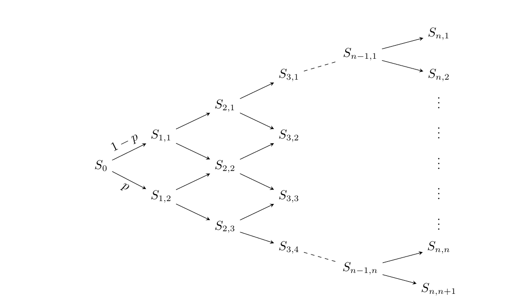
Underlying asset prices on an n-period binomial tree.

Figure 2.1 Underlying asset prices on an $n$-period binomial tree.

At each level, the nodes are numbered $i=1,\ldots,k+1$ in ascending order of stock price. The root node is denoted by $S_0$; the backward induction formulas use $S_{0,1}=S_0$ and $V_{0,1}=V_0$. If an upward branch represents a decline in stock price, then

\[ S_{k,i}=S_{k-1,i}d,\quad S_{k,i+1}=S_{k-1,i}u \tag{2.1.2} \]

Thus

\[ S_{k,i}=S_0d^{k+1-i}u^{i-1},\quad 0\leq k\leq n,\quad 1\leq i\leq k+1. \tag{2.1.3} \]

The CRR construction chooses the upward and downward factors so that the two possible changes in log stock price have the same magnitude:

\[ u=e^{\sigma\sqrt{h}} \tag{2.1.4} \]

\[ d=e^{-\sigma\sqrt{h}} \tag{2.1.5} \]

Thus $ud=1$, and the changes in log stock price at each step are $\sigma\sqrt{h}$ and $-\sigma\sqrt{h}$. Risk-neutral valuation requires the conditional mean of the next-period stock price on the tree to equal the stock price with risk-free growth, so

\[ p(uS_k)+(1-p)dS_k=S_ke^{rh}. \]

Rearranging gives the risk-neutral probability of an upward move:

\[ p=\frac{e^{rh}-d}{u-d} \tag{2.1.6} \]

The CRR Tree approximates the BSM model by matching the one-step conditional mean and conditional variance. Weighting the two possible next-period stock prices by their probabilities gives the conditional mean on the tree:

\[ \begin{aligned} \mathbb{E}_{\mathrm{CRR}}[S_{k+1}\mid S_k]&=p(uS_k)+(1-p)(dS_k)\\ &=S_k[pu+(1-p)d]\\ &=S_ke^{rh}. \end{aligned} \]

The last step follows from the risk-neutral probability in equation (2.1.6). The conditional mean under risk-neutral geometric Brownian motion also equals $S_ke^{rh}$. Given the stock price at time $kh$, denoted by $S_k$, the log stock price in the next period has the distribution

\[ \ln S_{k+1}\mid S_k\sim N\left(\ln S_k+\left(r-\frac{\sigma^2}{2}\right)h,\sigma^2h\right). \]

Based on the expectation of a Lognormal random variable, we get

\[ \mathbb{E}[S_{k+1}\mid S_k]=\exp\left\{\ln S_k+\left(r-\frac{\sigma^2}{2}\right)h+\frac{\sigma^2h}{2}\right\}=S_ke^{rh} \tag{2.1.7} \]

Thus, under the risk-neutral measure, the tree and geometric Brownian motion have the same conditional mean.

The conditional second moment and conditional variance of the next-period stock price on the tree are, respectively,

\[ \begin{aligned} \mathbb{E}_{\mathrm{CRR}}[S_{k+1}^2\mid S_k]&=S_k^2[pu^2+(1-p)d^2],\\ \operatorname{Var}_{\mathrm{CRR}}(S_{k+1}\mid S_k)&=\mathbb{E}_{\mathrm{CRR}}[S_{k+1}^2\mid S_k]-\mathbb{E}_{\mathrm{CRR}}[S_{k+1}\mid S_k]^2\\ &=S_k^2p(1-p)(u-d)^2. \end{aligned} \]

The conditional second moment and conditional variance of the next-period stock price under geometric Brownian motion are, respectively,

\[ \mathbb{E}[S_{k+1}^2\mid S_k]=\exp\left\{2\ln S_k+2\left(r-\frac{\sigma^2}{2}\right)h+\frac{4\sigma^2h}{2}\right\}=S_k^2e^{(2r+\sigma^2)h} \tag{2.1.8} \]

\[ \begin{aligned} \operatorname{Var}_{\mathrm{GBM}}(S_{k+1}\mid S_k)&=\mathbb{E}[S_{k+1}^2\mid S_k]-\mathbb{E}[S_{k+1}\mid S_k]^2\\ &=S_k^2e^{2rh}(e^{\sigma^2h}-1). \end{aligned} \tag{2.1.9} \]

At finite step sizes, the two conditional variances differ. As $h\to0$, they agree to first order in $h$, as the following expansions show.

First expand the binomial tree factors in equations (2.1.4) and (2.1.5):

\[ u-d=e^{\sigma\sqrt h}-e^{-\sigma\sqrt h}=2\sigma\sqrt h+O(h^{3/2}). \]

Hence \[ \lim_{h\to0}p=\frac12, \qquad \lim_{h\to0}\frac{u-d}{\sqrt h}=2\sigma. \] Dividing the tree’s conditional variance by $h$ and taking the limit gives \[ \lim_{h\to0}\frac{\operatorname{Var}_{\mathrm{CRR}}(S_{k+1}\mid S_k)}{h} =S_k^2\lim_{h\to0}p(1-p)\left(\frac{u-d}{\sqrt h}\right)^2 =S_k^2\sigma^2. \tag{2.1.10} \]

For the conditional variance under geometric Brownian motion, as $h\to0$, $e^{2rh}\to1$ and $(e^{\sigma^2h}-1)/h\to\sigma^2$, so \[ \lim_{h\to0}\frac{\operatorname{Var}_{\mathrm{GBM}}(S_{k+1}\mid S_k)}{h} =S_k^2\sigma^2. \tag{2.1.11} \]

These limits show that the CRR tree and geometric Brownian motion have the same conditional variance to first order in $h$.

Given the volatility $\sigma$, risk-free interest rate $r$, option maturity $T$, and number of tree steps $n$, Function 2.1 calculates the risk-neutral upward probability $p$ and the powers $u^i, d^i, i = 0, 1, . . . , n$. These powers give the asset prices at times $0, h, 2h, . . . , nh$ through equation (2.1.3).

From Formulas to Code

time_step corresponds to $h=T/n$; up, down, and up_probability correspond to $u$, $d$, and $p$ in equations (2.1.4)–(2.1.6), respectively.

down_values stores the powers $d^n,d^{n-1},\ldots,1$ in that order, and up_values stores $1,u,\ldots,u^n$. Multiplying the two arrays elementwise and scaling the result by $S_0$ gives the terminal stock prices $S_0d^{n-j}u^j$ in ascending order, where $j=0,\ldots,n$.

Function 2.1: CRR tree parameters

def crr_tree_parameters(model, maturity, n_steps):
    """Generate CRR down/up powers, the risk-neutral probability, and the time step."""
    time_step = maturity / n_steps
    up = np.exp(model.volatility * np.sqrt(time_step))
    down = 1.0 / up
    up_probability = (np.exp(model.rate * time_step) - down) / (up - down)
    down_values = down ** np.arange(n_steps, -1, -1)
    up_values = up ** np.arange(n_steps + 1)
    return down_values, up_values, up_probability, time_step

2.1.1 European Options

European option pricing starts with the binomial tree generated using Function 2.1. Backward induction from maturity $T$ then gives the option prices at times $(n-1)h,\ldots,h,0$. Let $g(S_T)$ denote the option payoff at maturity. Then

\[ V_{n,i}=g(S_{n,i}) \tag{2.1.12} \]

Working backward from maturity gives

\[ V_{k,i}=e^{-rh}\left((1-p)V_{k+1,i}+pV_{k+1,i+1}\right),\quad 0\leq k\leq n-1,\quad 1\leq i\leq k+1. \tag{2.1.13} \]

Equation (2.1.13) gives the value at each node in two steps. First, weighting the two successor values by the risk-neutral probabilities gives their conditional expectation. Multiplying this expectation by $e^{-rh}$ then discounts it to the current time. Backward induction starts at maturity, when the exercise payoff directly determines each node’s value. Once the values at one level are known, they determine the values at the preceding level. Repeating this recursion gives the option price at time 0.

Figure 2.2 illustrates how to price a European put option on a 2-period CRR binomial tree.

Generate the underlying asset prices on the binomial tree in the left panel of Figure 2.2.
At option maturity $T$, substitute the asset prices $S_0d^2,S_0,S_0u^2$ on the binomial tree into the European put option payoff at maturity $V=g(S_T)=(K-S_T)^+$ (right panel of Figure 2.2).
Calculate the option prices at time $T/2$.
Calculate the option price at time $0$.

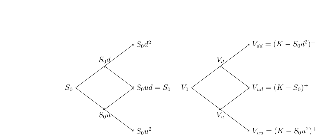
2-period CRR binomial tree. The left panel shows underlying asset prices on the binomial tree, and the right panel shows option prices on the binomial tree.

Figure 2.2 2-period CRR binomial tree. The left panel shows underlying asset prices on the binomial tree, and the right panel shows option prices on the binomial tree.

For this 2-period example, first substitute the terminal asset prices $S_0d^2,S_0,S_0u^2$ into the put payoff $(K-S_T)^+$. The values at the preceding level are then

\[ V_d=e^{-rT/2}\left[pV_{ud}+(1-p)V_{dd}\right] \tag{2.1.14} \]

\[ V_u=e^{-rT/2}\left[pV_{uu}+(1-p)V_{ud}\right] \tag{2.1.15} \]

Finally, the price at the root node is

\[ V_0=e^{-rT/2}\left[pV_u+(1-p)V_d\right]. \tag{2.1.16} \]

Function 2.2 implements CRR binomial tree pricing for European options. Higham (2002) describes further binomial tree implementations.

From Formulas to Code

discount_factor corresponds to the one-step discount factor $e^{-rh}$; values corresponds to the option values $V_{k,i}$ at the same level in equations (2.1.12)–(2.1.13).

The array values stores option values at the same level in ascending order of stock price. At each backward step, values[:i] and values[1:i+1] give the downward and upward successor values, respectively, for each node at the preceding level. Weighting and discounting each pair of adjacent values gives one value at the preceding level, reducing the array length from $i+1$ to $i$. At time 0, the array contains only the initial option price.

Function 2.2: European option pricing on a CRR tree

def european_crr_price(model, option, settings):
    """Generate terminal payoffs and discount backward through the European CRR tree."""
    n_steps = settings.n_steps
    down_values, up_values, up_probability, time_step = crr_tree_parameters(
        model, option.maturity, n_steps
    )
    values = np.maximum(
        option.cp * (option.spot * down_values * up_values - option.strike),
        0.0,
    )
    discount_factor = np.exp(-model.rate * time_step)
    for i in range(n_steps, 0, -1):
        values = discount_factor * (
            up_probability * values[1 : i + 1]
            + (1.0 - up_probability) * values[:i]
        )
    return float(values[0])

Table 2.1 compares CRR prices with the analytical values using $n=50$ steps. With underlying asset price $S_0=45$, volatility $\sigma=0.2$, interest rate $r=6\%$, strike prices $K=40,45,50$, and maturities $T=0.5,2$, the relative errors are approximately 1% or less.

# Table 2.1: European put prices with 50 CRR steps, S0=45, sigma=0.2, and r=6%
reference_steps = 50
reference_strikes = (40.0, 45.0, 50.0)
reference_maturities = (0.5, 2.0)

crr_reference_rows = []
for maturity in reference_maturities:
    for strike in reference_strikes:
        reference_option = EuropeanOption.put(
            spot=45.0, strike=strike, maturity=maturity
        )
        black_scholes_value = black_scholes_formula(
            model.volatility,
            reference_option.spot,
            reference_option.strike,
            reference_option.maturity,
            model.rate,
            reference_option.cp,
        )
        crr_value = european_crr_price(
            model,
            reference_option,
            replace(settings, n_steps=reference_steps),
        )
        crr_reference_rows.append(
            {
                "K": strike,
                "T": maturity,
                "V_BS": round(black_scholes_value, 4),
                "V_CRR": round(crr_value, 4),
                "Relative error (%)": round(
                    100
                    * abs(crr_value - black_scholes_value)
                    / black_scholes_value,
                    2,
                ),
            }
        )
pd.DataFrame(crr_reference_rows)

	K	T	V_BS	V_CRR	Relative error (%)
0	40.0	0.5	0.4510	0.4462	1.06
1	45.0	0.5	1.8902	1.8775	0.67
2	50.0	0.5	4.7620	4.7682	0.13
3	40.0	2.0	1.2562	1.2696	1.07
4	45.0	2.0	2.6503	2.6247	0.97
5	50.0	2.0	4.7038	4.7137	0.21

Table 2.1 European put prices from a CRR binomial tree with $n=50$ steps. Relative errors are expressed as percentages. The other option parameters are $S_0=45,\sigma=0.2,r=6\%$.

2.1.2 $\Delta$ and $\Gamma$ Estimation

A simple way to estimate sensitivity parameters with a binomial tree is to use finite differences: change a market risk factor, such as stock price or volatility, by a small amount, such as 1% or 1 basis point, and reprice the option. For $\Delta$ and $\Gamma$, more direct methods are available.

2.1.2.1 Hull’s Method

Hull (2014) shows that $\Delta$ and $\Gamma$ can be estimated directly on the binomial tree generated for pricing. The two nodes at time $h=T/n$ are used to estimate $\Delta$ at the current time, while the three nodes at time $2h$ are used to estimate $\Gamma$ at the current time. For the binomial tree nodes at times $0,h,2h$ shown in Figure 2.3, equations (2.1.17) and (2.1.18) give the estimates of $\Delta$ and $\Gamma$, respectively.

\[ \Delta=\frac{V_{1,2}-V_{1,1}}{S_{1,2}-S_{1,1}} \tag{2.1.17} \]

\[ \Gamma=\frac{\dfrac{V_{2,3}-V_{2,2}}{S_{2,3}-S_{2,2}}-\dfrac{V_{2,2}-V_{2,1}}{S_{2,2}-S_{2,1}}}{\dfrac12(S_{2,3}-S_{2,1})}. \tag{2.1.18} \]

Equation (2.1.17) divides the change in option value between two nodes by the change in stock price to obtain the local slope of the price curve, which is Delta. To calculate Gamma, first find the slopes of the left and right segments between the three nodes at time $2h$, then divide their difference by the corresponding stock price spacing. Each slope corresponds to the midpoint of its interval, and the distance between these midpoints is $\tfrac12(S_{2,3}-S_{2,1})$, so equation (2.1.18) uses this distance as the denominator.

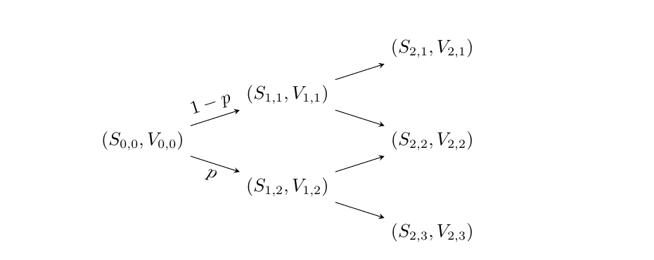
Binomial tree nodes at times 0, h, and 2h.

Figure 2.3 Binomial tree nodes at times $0,h,2h$. In the figure, $S_{0,0}$ and $V_{0,0}$ refer to the root node and correspond to $S_0$ and $V_0$ in the text.

Function 2.3 calculates European option $\Delta$ and $\Gamma$ under the Black–Scholes model using Hull’s method.

From Formulas to Code

p, q, and h correspond to the upward probability $p$, downward probability $1-p$, and time step $h$, respectively.

After the first loop, values stores the three option values at time $2h$, and spots stores the corresponding stock prices $S_0d^2,S_0,S_0u^2$. left_delta and right_delta correspond to the left and right segment slopes in the numerator of equation (2.1.18). After one more backward step, the two values in values are used for the Delta estimate in equation (2.1.17).

Function 2.3: Delta and Gamma estimation using Hull’s method

def crr_delta_gamma(model, option, settings):
    """Return the European option price, Delta, and Gamma using Hull's method."""
    n_steps = settings.n_steps
    down_values, up_values, p, h = crr_tree_parameters(
        model, option.maturity, n_steps
    )
    up, down = up_values[1], down_values[-2]
    q = 1.0 - p
    discount = np.exp(-model.rate * h)
    stock_prices = option.spot * down_values * up_values
    values = np.maximum(option.cp * (stock_prices - option.strike), 0.0)

    for _ in range(n_steps - 2):
        values = discount * (p * values[1:] + q * values[:-1])

    spots = option.spot * np.array([down**2, 1.0, up**2])
    left_delta = (values[1] - values[0]) / (spots[1] - spots[0])
    right_delta = (values[2] - values[1]) / (spots[2] - spots[1])
    gamma = (right_delta - left_delta) / ((spots[2] - spots[0]) / 2.0)

    values = discount * (p * values[1:] + q * values[:-1])
    delta = (values[1] - values[0]) / (option.spot * (up - down))
    value = discount * (p * values[1] + q * values[0])
    return float(value), float(delta), float(gamma)

We fix the current price $S_0=40$, time to maturity $T=0.5$, volatility $\sigma=0.2$, interest rate $r=6\%$, and number of tree steps $n=100$. Table 2.2 shows that Hull’s method provides fairly accurate $\Delta$ and $\Gamma$ estimates for European put options across different strike prices.

# Compare Hull's method with analytical Black-Scholes values across strikes
greek_strikes = (35.0, 40.0, 45.0, 50.0, 55.0)
hull_greek_rows = []
for strike in greek_strikes:
    strike_option = EuropeanOption.put(
        spot=option.spot, strike=strike, maturity=option.maturity
    )
    _, tree_delta, tree_gamma = crr_delta_gamma(model, strike_option, settings)
    exact_greeks = black_scholes_greeks(
        model.volatility,
        strike_option.spot,
        strike_option.strike,
        strike_option.maturity,
        model.rate,
        strike_option.cp,
    )
    hull_greek_rows.append(
        {
            "Strike": strike,
            "Tree Delta": round(tree_delta, 4),
            "Black–Scholes Delta": round(exact_greeks["delta"], 4),
            "Tree Gamma": round(tree_gamma, 4),
            "Black–Scholes Gamma": round(exact_greeks["gamma"], 4),
        }
    )
pd.DataFrame(hull_greek_rows)

	Strike	Tree Delta	Black–Scholes Delta	Tree Gamma	Black–Scholes Gamma
0	35.0	-0.1100	-0.1099	0.0334	0.0332
1	40.0	-0.3889	-0.3886	0.0683	0.0678
2	45.0	-0.7098	-0.7088	0.0608	0.0606
3	50.0	-0.9038	-0.9023	0.0302	0.0305
4	55.0	-0.9763	-0.9755	0.0099	0.0102

Table 2.2 Comparison of estimates from Hull’s method with Black–Scholes analytical values across strike prices.

2.1.2.2 Extended Binomial Tree

Pelsser and Vorst (1994) proposed an extended binomial tree that estimates $\Delta$ and $\Gamma$ using neighboring option values at the current time. As shown in Figure 2.4, the extended tree begins two periods before the current time ($-2h$). Here $S_{-1,1}=S_0d,S_{-1,2}=S_0u,S_{-2}=S_0$.

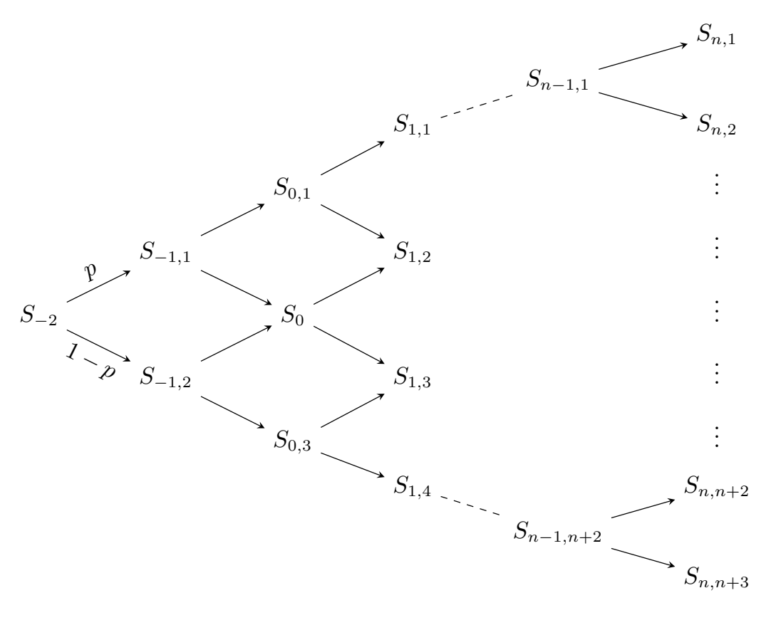
Extended binomial tree nodes at times −2h, −h, 0, and h.

Figure 2.4 Extended binomial tree nodes at times $-2h,-h,0,h$.

On the extended binomial tree, the estimates of $\Delta$ and $\Gamma$ are given by the following formulas.

\[ \Delta=\frac{V_{0,3}-V_{0,1}}{S_{0,3}-S_{0,1}} \tag{2.1.19} \]

\[ \Gamma=\frac{\dfrac{V_{0,3}-V_0}{S_{0,3}-S_0}-\dfrac{V_0-V_{0,1}}{S_0-S_{0,1}}}{\dfrac12(S_{0,3}-S_{0,1})}. \tag{2.1.20} \]

Extending the tree two periods backward gives three stock price nodes at time 0: $S_0d^2$, $S_0$, and $S_0u^2$. The options at all three nodes have the same remaining time to maturity $T$. Comparing the option values at these three stock prices therefore gives Delta and Gamma estimates at the current time. The middle node gives the required option price, while the nodes on either side provide the neighboring values needed to calculate the slope and curvature.

Function 2.4 calculates European option $\Delta$ and $\Gamma$ under the Black–Scholes model using an extended tree.

From Formulas to Code

total_steps=n_steps+2 is the total number of steps from $-2h$ to $T$. With a step size of $h=T/n$, after n_steps backward steps from the terminal level, the three option values at time 0 remain.

value_down, value, and value_up correspond to $V_{0,1}$, $V_0$, and $V_{0,3}$ in equations (2.1.19)–(2.1.20), respectively, with corresponding stock prices $S_0d^2,S_0,S_0u^2$.

Function 2.4: Delta and Gamma estimation on an extended tree

def crr_extended_delta_gamma(model, option, settings):
    """Return the European option price, Delta, and Gamma using an extended CRR tree."""
    n_steps = settings.n_steps
    down_values, up_values, p, h = crr_tree_parameters(
        model, option.maturity, n_steps
    )
    up, down = up_values[1], down_values[-2]
    q = 1.0 - p
    discount = np.exp(-model.rate * h)

    total_steps = n_steps + 2
    up_moves = np.arange(total_steps + 1)
    stock_prices = option.spot * down ** (total_steps - up_moves) * up**up_moves
    values = np.maximum(option.cp * (stock_prices - option.strike), 0.0)
    for _ in range(n_steps):
        values = discount * (p * values[1:] + q * values[:-1])

    value_down, value, value_up = values
    delta = (value_up - value_down) / (option.spot * (up**2 - down**2))
    gamma = 2.0 * (
        (value_up - value) / (up**2 - 1.0)
        - (value - value_down) / (1.0 - down**2)
    ) / (option.spot**2 * (up**2 - down**2))
    return float(value), float(delta), float(gamma)

Here, the current price $S_0=40$, time to maturity $T=0.5$, volatility $\sigma=0.2$, interest rate $r=6\%$, and number of tree steps $n=100$ are held fixed. Table 2.3 shows that the extended binomial tree also provides fairly accurate $\Delta$ and $\Gamma$ estimates for European put options across different strike prices.

# Compare the extended tree with analytical Black-Scholes values across strikes
greek_strikes = (35.0, 40.0, 45.0, 50.0, 55.0)
extended_greek_rows = []
for strike in greek_strikes:
    strike_option = EuropeanOption.put(
        spot=option.spot, strike=strike, maturity=option.maturity
    )
    _, tree_delta, tree_gamma = crr_extended_delta_gamma(model, strike_option, settings)
    exact_greeks = black_scholes_greeks(
        model.volatility,
        strike_option.spot,
        strike_option.strike,
        strike_option.maturity,
        model.rate,
        strike_option.cp,
    )
    extended_greek_rows.append(
        {
            "Strike": strike,
            "Tree Delta": round(tree_delta, 4),
            "Black–Scholes Delta": round(exact_greeks["delta"], 4),
            "Tree Gamma": round(tree_gamma, 4),
            "Black–Scholes Gamma": round(exact_greeks["gamma"], 4),
        }
    )
pd.DataFrame(extended_greek_rows)

	Strike	Tree Delta	Black–Scholes Delta	Tree Gamma	Black–Scholes Gamma
0	35.0	-0.1115	-0.1099	0.0333	0.0332
1	40.0	-0.3884	-0.3886	0.0676	0.0678
2	45.0	-0.7065	-0.7088	0.0606	0.0606
3	50.0	-0.9008	-0.9023	0.0307	0.0305
4	55.0	-0.9749	-0.9755	0.0103	0.0102

Table 2.3 Comparison of extended binomial tree estimates with Black–Scholes analytical values across strike prices.

The next experiment varies the number of tree steps and calculates the errors of both methods relative to the Black–Scholes analytical Greeks. The step counts are $20,40,\ldots,10240$, allowing a comparison of how the errors change as the tree is refined.

# Calculate intermediate results using the parameters and formulas above
greek_option = option

greek_steps = np.array(
    [20, 40, 80, 160, 320, 640, 1280, 2560, 5120, 10240]
)
bs_greeks = black_scholes_greeks(
    model.volatility,
    greek_option.spot,
    greek_option.strike,
    greek_option.maturity,
    model.rate,
    greek_option.cp,
)
hull_results = np.array(
    [
        crr_delta_gamma(
            model,
            greek_option,
            replace(settings, n_steps=int(steps)),
        )[1:]
        for steps in greek_steps
    ]
)
extended_results = np.array(
    [
        crr_extended_delta_gamma(
            model,
            greek_option,
            replace(settings, n_steps=int(steps)),
        )[1:]
        for steps in greek_steps
    ]
)
delta_errors = {
    "Hull's method": hull_results[:, 0] - bs_greeks["delta"],
    "Extended tree": extended_results[:, 0] - bs_greeks["delta"],
}
gamma_errors = {
    "Hull's method": hull_results[:, 1] - bs_greeks["gamma"],
    "Extended tree": extended_results[:, 1] - bs_greeks["gamma"],
}

Figure 2.5 compares the Delta estimation errors of the two methods using the same parameters. The curves show signed errors, so accuracy is measured by distance from the zero line. The horizontal axis uses a logarithmic scale to show small and large step counts on the same plot.

# Figure 2.5: European put Delta errors using Hull's method and the extended tree
fig, ax = plt.subplots(figsize=(7.5, 4.2))
delta_styles = {
    "Hull's method": {"color": "tab:blue", "marker": "D"},
    "Extended tree": {"color": "tab:orange", "marker": "o"},
}
for label, errors in delta_errors.items():
    ax.semilogx(
        greek_steps,
        errors,
        linestyle="-",
        linewidth=1.1,
        markersize=4.5,
        label=label,
        **delta_styles[label],
    )
ax.axhline(0.0, color="black", linewidth=0.8, alpha=0.6)
ax.set_xlim(10, 10240)
ax.set_ylim(-0.006, 0.012)
ax.set_xlabel("Binomial steps $n$")
ax.set_ylabel("Delta error")
ax.set_title("Binomial tree Delta error")
ax.legend(frameon=False)
ax.grid(True, which="both", alpha=0.25)
fig.tight_layout()
plt.show()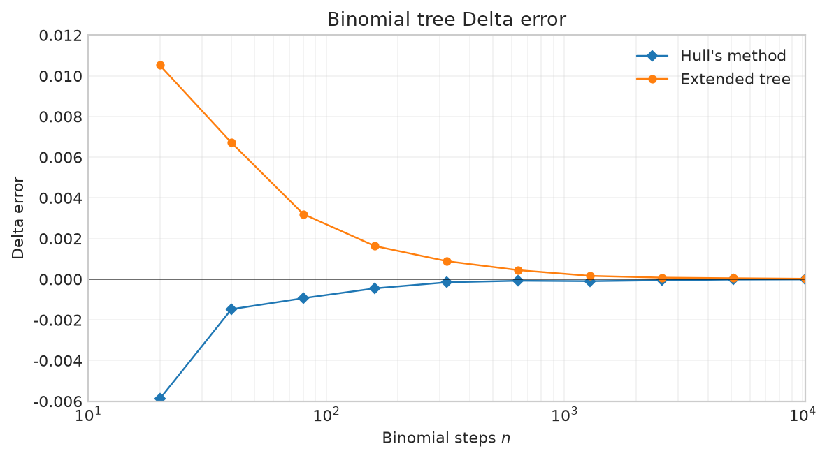

Figure 2.5 Errors in estimating European put option Delta using Hull's method and the extended binomial tree.

Figure 2.5 Errors in estimating European put option Delta using Hull’s method and the extended binomial tree.

Hull’s method has smaller absolute Delta errors at all ten plotted step counts.

Hull’s Delta estimate uses the nodes $S_0d$ and $S_0u$ at time $h$, whereas the extended-tree estimate uses $S_0d^2$ and $S_0u^2$ at time 0. Their stock-price spacings are

\[ \begin{aligned} w_H &= S_0(u-d),\\ w_E &= S_0(u^2-d^2),\\ \frac{w_E}{w_H} &= u+d=e^{\sigma\sqrt{h}}+e^{-\sigma\sqrt{h}}\approx 2. \end{aligned} \]

For small $h$, the extended tree therefore uses approximately twice the stock-price spacing for Delta. Its neighboring option values have the same remaining maturity $T$, while Hull’s values have remaining maturity $T-h$. The extended tree removes this time shift, but its wider interval averages the slope over a broader range of stock prices and changes the spatial finite-difference bias.

In this example, Hull’s time and spacing approximation bias partly cancels the error in the CRR node values, while the extended tree’s spatial approximation bias and node-value error reinforce each other.

Figure 2.6 compares Gamma estimation errors using the same option parameters and step counts.

# Figure 2.6: European put Gamma errors using Hull's method and the extended tree
fig, ax = plt.subplots(figsize=(7.5, 4.2))
gamma_styles = {
    "Hull's method": {"color": "tab:blue", "marker": "D"},
    "Extended tree": {"color": "tab:orange", "marker": "o"},
}
for label, errors in gamma_errors.items():
    ax.semilogx(
        greek_steps,
        errors,
        linestyle="-",
        markersize=4.5,
        label=label,
        **gamma_styles[label],
    )
ax.axhline(0.0, color="black", linewidth=0.8, alpha=0.6)
ax.set_xlim(10, 20000)
ax.set_ylim(-0.0006, 0.0008)
ax.set_xlabel("Binomial steps $n$")
ax.set_ylabel("Gamma error")
ax.set_title("Binomial tree Gamma error")
ax.legend(frameon=False)
ax.grid(True, which="both", alpha=0.25)
fig.tight_layout()
plt.show()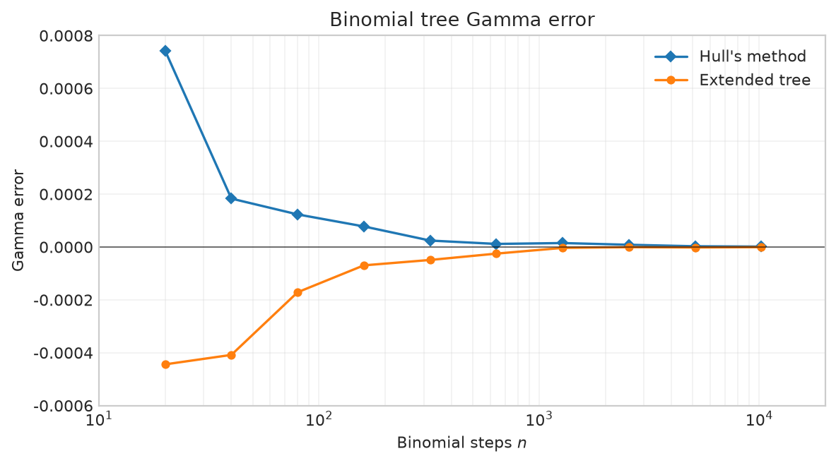

Figure 2.6 Errors in estimating European put option Gamma using Hull's method and the extended binomial tree.

Figure 2.6 Errors in estimating European put option Gamma using Hull’s method and the extended binomial tree.

Hull’s method has smaller absolute errors at $n=40,80,320,640$, while the extended tree has smaller absolute errors at the other six plotted step counts. Both methods converge toward the analytical Gamma as the tree is refined; their accuracy ranking changes with the step count.

2.1.3 American Options

American options allow the holder to exercise at any time before maturity $T$, so pricing requires deciding when to exercise and when to keep holding the option. Even under the BSM model, American option prices generally have no analytical expression and must be approximated numerically.

Dividing the time to maturity $T$ into $n$ equal intervals and allowing exercise only at times $0,h,2h,\ldots,nh$ defines a Bermudan option. It lies between a European option, which can only be exercised at maturity, and an American option, which can be exercised continuously; as $n$ increases, the Bermudan option price provides an approximation to the American option price. In the following calculations, we refer to these contracts that allow early exercise as American options.

Let $g(S)$ denote the exercise payoff and $\mathcal T_n$ the set of stopping times taking values in $\{0,h,2h,\ldots,nh\}$. Each stopping time represents an exercise rule based on information available at that time, such as exercising when the stock price first enters the exercise region. The initial option value on the discrete exercise grid can be written as

\[ \begin{align*} V(0,S) = \sup_{\tau\in\mathcal T_n}\mathbb{E}^Q\left[e^{-r\tau}g(S_\tau)\mid S_0=S\right]. \tag{2.1.21} \end{align*} \]

Since an American option can be exercised at any permitted time, its value must be at least as large as the exercise payoff. Thus, at each permitted exercise time $t$,

\[ V(t,S)\geq g(S). \tag{2.1.22} \]

American call options without dividends

Assume that the underlying asset pays no dividends and that the risk-free interest rate satisfies $r\geq0$.

First, because an American option can be exercised early, its value must be at least as large as the value of the corresponding European option, as expressed by

\[ \begin{align*} C_A(S_t,T-t,K) \geq C_E(S_t,T-t,K). \tag{2.1.23} \end{align*} \]

where $S_t$ is the underlying asset price at time $t$, $K$ is the strike price of the European and American options, and $T$ is the maturity.

Second, in the absence of dividends, the lower bound on the European option price is

\[ \begin{align*} C_E(S_t,T-t,K) \geq \left(S_t-Ke^{-r(T-t)}\right)^+. \tag{2.1.24} \end{align*} \]

To derive equation (2.1.24), we compare two portfolios at time $t$:

Portfolio 1: one European call option $C_E(S,T-t,K)$ and cash $Ke^{-r(T-t)}$;
Portfolio 2: one share of stock $S$.

The table below shows the values of these two portfolios at option maturity $T$.

	$S_T<K$	$S_T\geq K$
Portfolio 1	$K$	$(S_T-K)+K=S_T$
Portfolio 2	$S_T$	$S_T$

Table 2.4 Comparison of the two portfolios at maturity in the proof of the price lower bound for a call option without dividends.

At maturity, Portfolio 1 is worth more than Portfolio 2 when $S_T<K$, and has the same value as Portfolio 2 when $S_T\geq K$. Therefore, Portfolio 1 must also be worth at least as much as Portfolio 2 at time $t$, that is,

\[ \begin{align*} C_E(S_t,T-t,K)+Ke^{-r(T-t)}\geq S_t. \tag{2.1.25} \end{align*} \]

Moving $Ke^{-r(T-t)}$ to the right-hand side of the inequality, and using the fact that option prices are always nonnegative, gives inequality (2.1.24). Combining this with inequality (2.1.23) gives

\[ \begin{align*} C_A(S_t,T-t,K)\geq\left(S_t-Ke^{-r(T-t)}\right)^+. \tag{2.1.26} \end{align*} \]

Finally, at any permitted exercise time $\tau\leq T$, the immediate exercise payoff is $(S_\tau-K)^+$. The value of holding the option until maturity equals the price of the corresponding European call option. From $r\geq0$ and equation (2.1.24),

\[ \begin{align*} \underbrace{(S_\tau-K)^+}_{\text{stop (exercise) value}}\leq\left(S_\tau-Ke^{-r(T-\tau)}\right)^+\leq\underbrace{C_E(S_\tau,T-\tau,K)}_{\text{hold value until maturity}}, \tag{2.1.27} \end{align*} \]

Thus, holding until maturity is worth at least as much as exercising immediately. Holding remains an available choice at every permitted exercise time, so $\tau=T$ can be chosen as the optimal exercise rule. Therefore, with no dividends and $r\geq0$, an American call option has the same price as the corresponding European call option.

Pricing American options using dynamic programming

The no-early-exercise argument above does not extend to American calls on dividend-paying assets or to American puts. Exercising a call allows the holder to own the stock and receive subsequent dividends; exercising a put brings forward receipt of the strike, allowing that cash to earn interest. These benefits can make early exercise optimal, so we cannot price these options simply by using the corresponding European prices. Their prices generally have no closed-form expression under the BSM model, so we compute them numerically using dynamic programming.

Dynamic programming calculates the American option price in equation (2.1.21) by working backward from maturity $t=nh$ to $t=0$. Let $V_i(x)=V(ih,x)$ denote the option value when $S_{ih}=x$ and the option has not yet been exercised at $t=ih$. Then

\[ \begin{align*} V_n(x) ={}& g_n(x), \tag{2.1.28}\\ V_{i-1}(x) ={}& \max\left\{g_{i-1}(x),e^{-rh}\mathbb{E}^Q\left[V_i(S_{ih})\mid S_{(i-1)h}=x\right]\right\}, \tag{2.1.29}\\ & i=1,2,\ldots,n. \tag{2.1.30} \end{align*} \]

Here $g_{i-1}(x)$ is the exercise value at time $(i-1)h$, while $e^{-rh}\mathbb{E}^Q[V_i(S_{ih})\mid S_{(i-1)h}=x]$ is the continuation value at time $(i-1)h$. At each step, the American option value is the larger of these two values. Exercise is optimal when the exercise value exceeds the continuation value; otherwise, holding the option is optimal.

For example, consider an American put option with a strike price of 40 at a node where the stock price is 30. Immediate exercise yields 10. If the continuation value at that node is 9.6, the optimal decision is to exercise, giving a node value of 10; if the continuation value is 10.4, the optimal decision is to hold the option, giving a node value of 10.4. The continuation value is calculated from the next-period option values, which already reflect the optimal exercise decisions at subsequent nodes. Working backward level by level therefore incorporates future exercise decisions into the current price.

Implementing dynamic programming on a CRR binomial tree

To implement the dynamic-programming recursion in equations (2.1.28)-(2.1.30), we need to evaluate the conditional expectation at each step. On a CRR binomial tree, each node has two possible next-period states, so this expectation becomes a weighted average of the two successor option values, with risk-neutral probabilities $p$ and $1-p$. Starting from the maturity payoffs, we work backward through the tree, discount this average to obtain the continuation value, and compare it with the immediate exercise value at each node.

Let the immediate exercise payoff of an American put option be $(K-S)^+$. At each binomial tree node where exercise is permitted, the recursion compares the immediate exercise value with the continuation value and takes the larger of the two. Thus, the American put option price is

\[ V_{k,i}=\max\left((K-S_{k,i})^+,e^{-rh}\left((1-p)V_{k+1,i}+pV_{k+1,i+1}\right)\right), \quad 0\leq k\leq n-1,\quad 1\leq i\leq k+1. \tag{2.1.31} \]

For the 2-period example shown in Figure 2.2, this gives

\[ V_d=\max\left((K-S_0d)^+,e^{-rT/2}\left[pV_{ud}+(1-p)V_{dd}\right]\right) \tag{2.1.32} \]

\[ V_u=\max\left((K-S_0u)^+,e^{-rT/2}\left[pV_{uu}+(1-p)V_{ud}\right]\right) \tag{2.1.33} \]

\[ V_0=\max\left((K-S_0)^+,e^{-rT/2}\left[pV_u+(1-p)V_d\right]\right). \tag{2.1.34} \]

Function 2.5 implements this recursion on a CRR tree.

From Formulas to Code

At each backward step, stock_prices stores the stock prices at the preceding level, for which option values are currently being calculated; exercise corresponds to the immediate exercise payoff $g(S)$ at these nodes, and continuation corresponds to the discounted conditional expectation of the next-period value. values = np.maximum(exercise, continuation) implements the nodewise maximum operation in equation (2.1.31).

Function 2.5: American option pricing on a CRR tree

def american_crr_price(model, option, settings):
    """Compare exercise and discounted continuation values at each American CRR level."""
    n_steps = settings.n_steps
    down_values, up_values, up_probability, time_step = crr_tree_parameters(
        model, option.maturity, n_steps
    )
    values = np.maximum(
        option.cp * (option.spot * down_values * up_values - option.strike),
        0.0,
    )
    discount_factor = np.exp(-model.rate * time_step)
    for i in range(n_steps, 0, -1):
        continuation = discount_factor * (
            up_probability * values[1 : i + 1]
            + (1.0 - up_probability) * values[:i]
        )
        stock_prices = (
            option.spot * down_values[n_steps - i + 1 :] * up_values[:i]
        )
        exercise = np.maximum(
            option.cp * (stock_prices - option.strike), 0.0
        )
        values = np.maximum(exercise, continuation)
    return float(values[0])

The next cell calls the American CRR pricing function and compares the result with the European put option price using the same parameters.

# Compare European and American prices for the same put option
european_put = european_crr_price(model, option, settings)
american_option = AmericanOption.put(
    spot=option.spot,
    strike=option.strike,
    maturity=option.maturity,
)
american_put = american_crr_price(model, american_option, settings)
early_exercise_premium = american_put - european_put
pd.Series(
    {
        "European put": european_put,
        "American put": american_put,
        "Early exercise premium": early_exercise_premium,
    }
)

European put              4.630949
American put              5.143206
Early exercise premium    0.512256
dtype: float64

2.1.4 Convergence Properties of the CRR Binomial Tree

Cox–Ross–Rubinstein (1979) showed that as the number of steps $n$ in a CRR binomial tree increases, the estimated European option price converges to the Black–Scholes price. F. Diener and M. Diener (2004) studied price oscillations in the CRR tree and found that the pricing error in typical binomial tree models is $O(1/n)$. The asymptotic error scales inversely with the number of steps: doubling $n$ roughly halves the CRR pricing error.

We first consider an at-the-money option and choose the parameters $S_0=K=10,T=1,\sigma=0.3,r=6\%$.

Plotting helper: CRR price convergence

def plot_crr_price_convergence(steps, prices, reference_price):
    """Plot CRR prices and the Black-Scholes benchmark, separating odd and even step counts."""
    odd_mask = steps % 2 == 1
    even_mask = ~odd_mask
    fig, plot_axes = plt.subplots(2, 1, figsize=(8.5, 7.0), sharex=True)
    plot_axes[0].plot(steps, prices, color="tab:blue", linewidth=1.0, label="CRR price")
    plot_axes[0].axhline(
        reference_price, color="tab:red", linewidth=1.2,
        label="Black–Scholes price",
    )
    plot_axes[0].set_ylabel("Option price")
    plot_axes[0].set_title("All step counts")
    plot_axes[0].legend(frameon=False)
    plot_axes[0].grid(True, alpha=0.25)

    plot_axes[1].plot(
        steps[odd_mask], prices[odd_mask], color="tab:green", linewidth=1.2,
        label="CRR price: odd n",
    )
    plot_axes[1].plot(
        steps[even_mask], prices[even_mask], color="tab:blue", linewidth=1.2,
        label="CRR price: even n",
    )
    plot_axes[1].axhline(
        reference_price, color="tab:red", linewidth=1.2,
        label="Black–Scholes price",
    )
    plot_axes[1].set_xlabel("Binomial steps $n$")
    plot_axes[1].set_ylabel("Option price")
    plot_axes[1].set_title("Odd and even step counts")
    plot_axes[1].legend(frameon=False)
    plot_axes[1].grid(True, alpha=0.25)
    fig.tight_layout()
    plt.show()

# Use sigma=0.3 for this section; the default model is used in the preceding examples
convergence_model = replace(model, volatility=0.30)
# Calculate intermediate results using the parameters and formulas above
atm_option = EuropeanOption.put(spot=10.0, strike=10.0, maturity=1.0)
convergence_steps = np.arange(50, 501)
bs_atm = black_scholes_formula(
    convergence_model.volatility,
    atm_option.spot,
    atm_option.strike,
    atm_option.maturity,
    convergence_model.rate,
    atm_option.cp,
)
crr_atm_prices = np.array(
    [
        european_crr_price(
            convergence_model,
            atm_option,
            replace(settings, n_steps=int(steps)),
        )
        for steps in convergence_steps
    ]
)
crr_atm_errors = np.abs(crr_atm_prices - bs_atm)
odd_mask = convergence_steps % 2 == 1
even_mask = convergence_steps % 2 == 0

With the parameters in this example and step counts $n=50,51,\ldots,500$, Figure 2.7 shows the following:

As the number of CRR steps increases from 50 to 500, the option prices oscillate around the Black–Scholes price.
With even step counts, the CRR tree consistently underestimates the option price, providing a lower bound.
With odd step counts, it consistently overestimates the option price, providing an upper bound.

# Figure 2.7: CRR at-the-money European put convergence for odd and even step counts
plot_crr_price_convergence(convergence_steps, crr_atm_prices, bs_atm)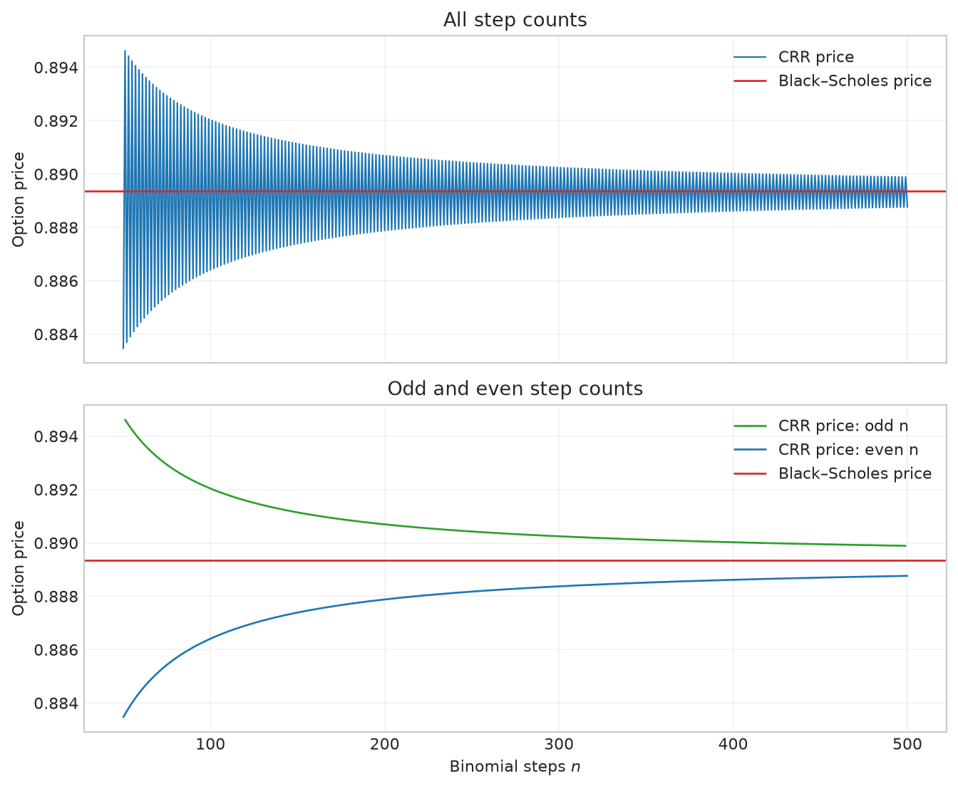

$Figure 2.7 At-the-money European put option prices obtained from CRR binomial trees with varying numbers of steps. The option parameters are $S_0=K=10,T=1,\sigma=0.3,r=6\%$.$

Figure 2.7 At-the-money European put option prices obtained from CRR binomial trees with varying numbers of steps. The option parameters are $S_0=K=10,T=1,\sigma=0.3,r=6\%$.

Figure 2.8 shows that the CRR pricing error converges monotonically to zero at a rate of $1/n$ when only even step counts are used. Using only odd step counts gives a similar result.

# Figure 2.8: CRR at-the-money European put errors for odd and even step counts
fig, ax = plt.subplots(figsize=(8.0, 5.2))
ax.loglog(
    convergence_steps[odd_mask],
    crr_atm_errors[odd_mask],
    "o",
    markersize=3.0,
    label="CRR error: odd n",
)
ax.loglog(
    convergence_steps[even_mask],
    crr_atm_errors[even_mask],
    "o",
    markersize=3.0,
    label="CRR error: even n",
)
ax.loglog(
    convergence_steps,
    crr_atm_errors[0] * (convergence_steps[0] / convergence_steps),
    "r-",
    linewidth=1.2,
    label="$1/n$",
)
ax.set_xlabel("Binomial steps $n$")
ax.set_ylabel("Absolute price error")
ax.set_title("CRR at-the-money put error")
ax.legend(frameon=False)
ax.grid(True, which="both", alpha=0.25)
fig.tight_layout()
plt.show()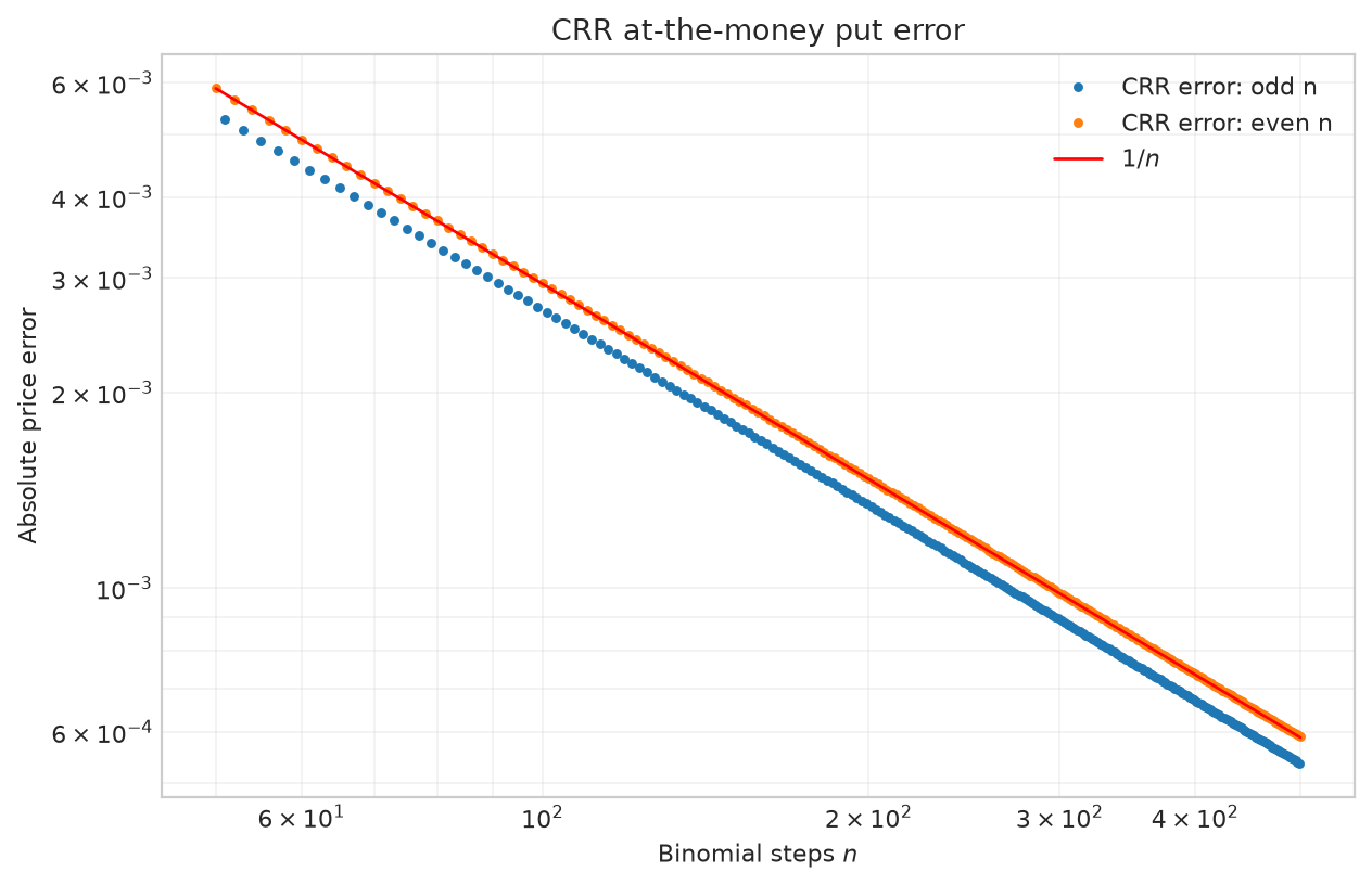

$Figure 2.8 Blue and orange dots represent the absolute pricing errors for the at-the-money European put option for odd and even step counts, respectively. The red solid line converges to 0 at a rate of $1/n$. The option parameters are $S_0=K=10,T=1,\sigma=0.3,r=6\%$.$

Figure 2.8 Blue and orange dots represent the absolute pricing errors for the at-the-money European put option for odd and even step counts, respectively. The red solid line converges to 0 at a rate of $1/n$. The option parameters are $S_0=K=10,T=1,\sigma=0.3,r=6\%$.

For options that are not at the money, the price curves for odd and even step counts also exhibit oscillations. For the in-the-money option example, set the current stock price to $S_0=8$ and use $K=10,T=1,\sigma=0.3,r=6\%$, again treating odd and even step counts as separate groups.

# Calculate intermediate results using the parameters and formulas above
itm_option = EuropeanOption.put(spot=8.0, strike=10.0, maturity=1.0)
bs_itm = black_scholes_formula(
    convergence_model.volatility,
    itm_option.spot,
    itm_option.strike,
    itm_option.maturity,
    convergence_model.rate,
    itm_option.cp,
)
crr_itm_prices = np.array(
    [
        european_crr_price(
            convergence_model,
            itm_option,
            replace(settings, n_steps=int(steps)),
        )
        for steps in convergence_steps
    ]
)
crr_itm_errors = np.abs(crr_itm_prices - bs_itm)

Figure 2.9 shows that the CRR option price estimates oscillate around the Black–Scholes price as $n$ increases, even when odd and even step counts are considered separately.

# Figure 2.9: CRR in-the-money European put convergence for odd and even step counts
plot_crr_price_convergence(convergence_steps, crr_itm_prices, bs_itm)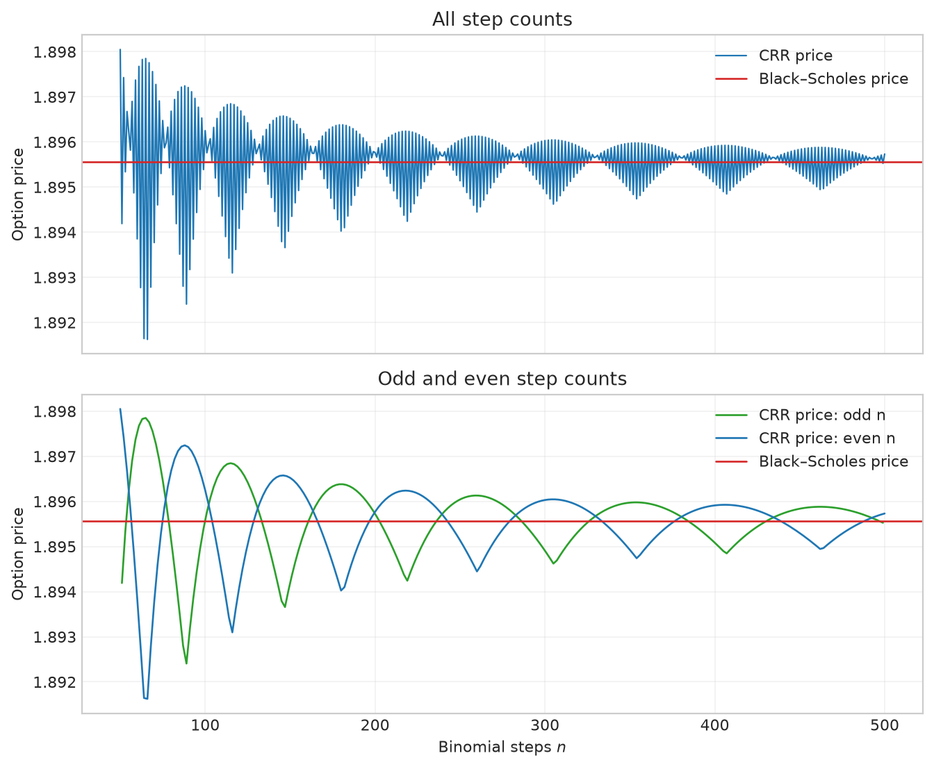

$Figure 2.9 In-the-money European put option prices obtained from CRR binomial trees with varying numbers of steps. The option parameters are $S_0=8,K=10,T=1,\sigma=0.3,r=6\%$.$

Figure 2.9 In-the-money European put option prices obtained from CRR binomial trees with varying numbers of steps. The option parameters are $S_0=8,K=10,T=1,\sigma=0.3,r=6\%$.

Figure 2.10 shows that the CRR error still converges at a rate of $1/n$, but fluctuates substantially as the step count increases.

# Figure 2.10: CRR in-the-money European put errors for odd and even step counts
fig, ax = plt.subplots(figsize=(8.0, 5.2))
ax.loglog(
    convergence_steps[odd_mask],
    crr_itm_errors[odd_mask],
    ":",
    linewidth=1.2,
    color="black",
    label="CRR error: odd n",
)
ax.loglog(
    convergence_steps[even_mask],
    crr_itm_errors[even_mask],
    "-",
    linewidth=1.2,
    color="tab:red",
    label="CRR error: even n",
)
ax.loglog(
    convergence_steps,
    crr_itm_errors[0] * (convergence_steps[0] / convergence_steps),
    "--",
    color="tab:blue",
    linewidth=1.2,
    label="$1/n$",
)
ax.set_xlabel("Binomial steps $n$")
ax.set_ylabel("Absolute price error")
ax.set_title("CRR in-the-money put error")
ax.legend(frameon=False)
ax.grid(True, which="both", alpha=0.25)
fig.tight_layout()
plt.show()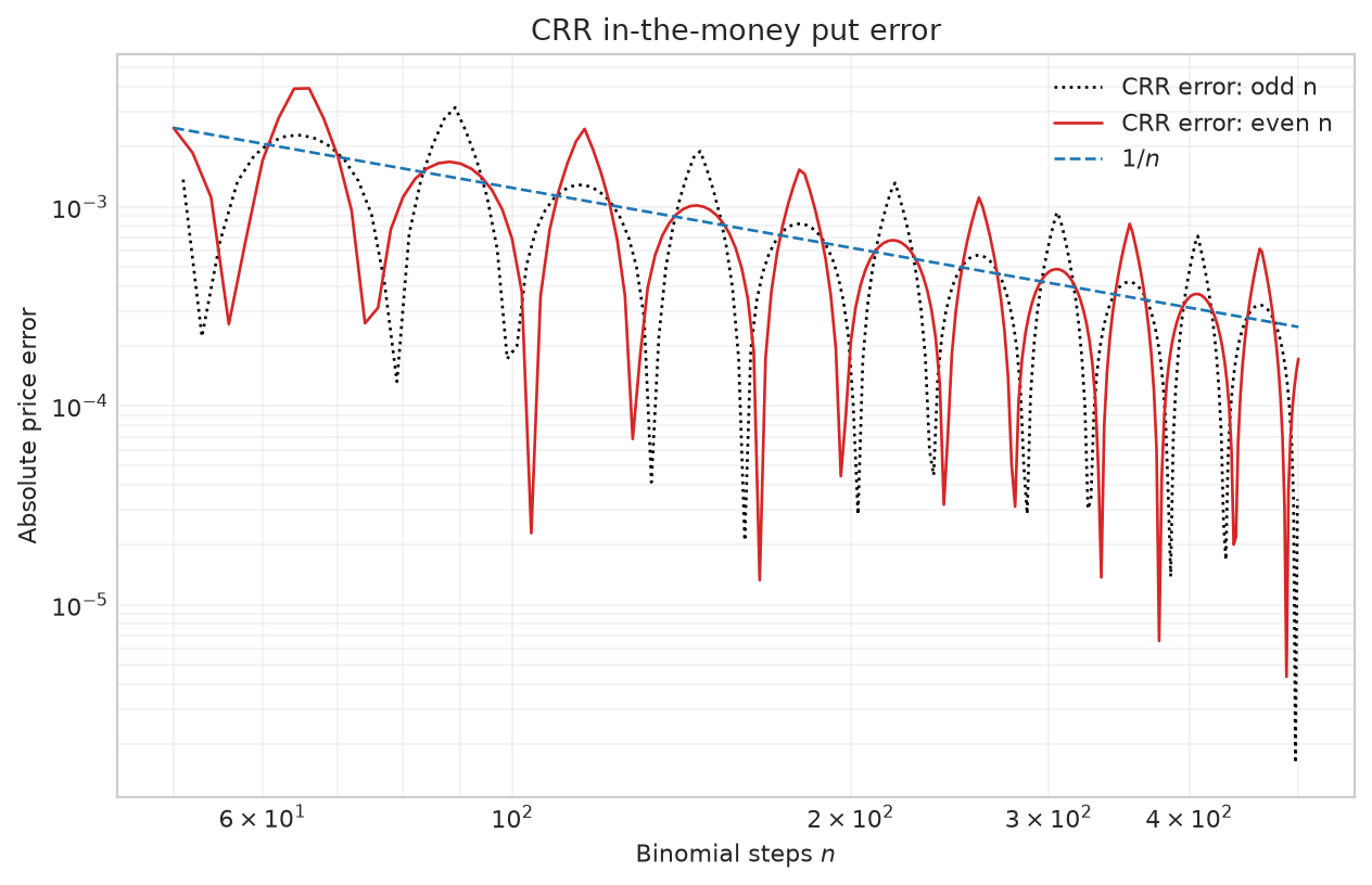

$Figure 2.10 The black dotted line and red solid line represent the absolute pricing errors for the in-the-money European put option for odd and even step counts, respectively. The blue dashed line converges to 0 at a rate of $1/n$. The option parameters are $S_0=8,K=10,T=1,\sigma=0.3,r=6\%$.$

Figure 2.10 The black dotted line and red solid line represent the absolute pricing errors for the in-the-money European put option for odd and even step counts, respectively. The blue dashed line converges to 0 at a rate of $1/n$. The option parameters are $S_0=8,K=10,T=1,\sigma=0.3,r=6\%$.

The pricing error of the CRR binomial tree comes from two sources:

The BSM model assumes that asset log returns follow a normal distribution, while the CRR binomial tree approximates the normal distribution with a discrete binomial distribution.
The position of the strike price $K$ relative to the terminal tree nodes $S_{n,i},i=1,\ldots,n+1$.

Increasing the number of binomial tree steps $n$ reduces the first type of error; by the central limit theorem, as $n\rightarrow\infty$, the distribution of log returns on the tree converges to the corresponding normal distribution. Figures 2.7 and 2.9 show that the second type of error is smaller for at-the-money options.

Figure 2.11 illustrates the effect of the strike position. Consider the 2-period and 4-period trees with parameters $S_0=8,T=1,\sigma=0.3,r=6\%$. For an at-the-money put, $K=S_0=8$ lies on a terminal node in both trees because their step counts are even (2 and 4). For an in-the-money option with $K=10$, however, when $n=2$, $K$ lies approximately midway between the two nodes 8 and 12.23, whereas for $n=4$, the distance from $K$ to the node at 10.80 is about 0.80, less than the distance of 2 to the node at 8. Thus, for options that are not at the money, changing $n$ changes the position of $K$ relative to the binomial tree nodes, causing the pricing error to oscillate.

The strike price has a pronounced effect on the error because the put option payoff at maturity $(K-S)^+$ has a kink at $S=K$: the slope on the left is $-1$ and the slope on the right is 0. The tree calculates expectations by weighting the payoffs at discrete nodes by their probabilities. When the number of steps changes, both the positions of nodes near the kink and the side of the kink on which they fall change, causing the pricing error to fluctuate.

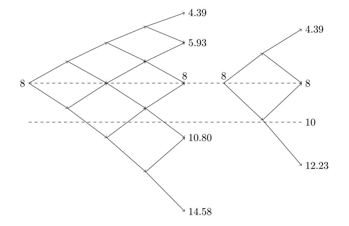
2-period and 4-period CRR binomial trees.

Figure 2.11 2-period and 4-period CRR binomial trees. The option parameters are $S_0=8,T=1,\sigma=0.3,r=6\%$.

Following the binomial tree method for option pricing proposed by Cox–Ross–Rubinstein (1979), many researchers developed improvements, including Broadie and Detemple (1996), Leisen and Reimer (1996), Tian (1993, 1999), Chung and Shih (2007), Boyle (1986), and Kamrad and Ritchken (1991). In addition, Joshi (2009) compared the performance of various binomial trees for pricing American options, while Chan et al. (2009) compared various trinomial trees. The following sections focus on three of these improvements: the flexible binomial tree proposed by Tian (1999), the binomial Black–Scholes tree proposed by Broadie and Detemple (1996), and the trinomial tree proposed by Boyle (1986).

2.2 Flexible Binomial Tree

To reduce the oscillations that occur as CRR binomial tree prices converge, Tian (1999) proposed a flexible binomial tree that places the strike price $K$ on a terminal node at maturity $T$. The CRR condition $ud=1$ can be relaxed by introducing a tilt parameter $\lambda$. Multiplying both the upward and downward CRR factors by $e^{\lambda\sigma^2h}$ shifts the terminal nodes so that one node lies at $K$. The adjusted factors and risk-neutral probability are

\[ u=e^{\sigma\sqrt h+\lambda\sigma^2h},\qquad d=e^{-\sigma\sqrt h+\lambda\sigma^2h},\qquad p=\frac{e^{rh}-d}{u-d}. \tag{2.2.1} \]

When $\lambda=0$, the flexible binomial tree reduces to the CRR binomial tree. When $\lambda>0$, asset prices on the binomial tree are higher than those on the CRR binomial tree; conversely, when $\lambda<0$, asset prices on the binomial tree are lower than those on the CRR binomial tree (for example, Figures 2.11 and 2.12 show 4-period binomial trees with $\lambda=0$ and $\lambda<0$, respectively).

In terms of log stock prices, the tilt parameter adds $\lambda\sigma^2h$ to both the upward and downward log factors, while the distance between them remains $\log u-\log d=2\sigma\sqrt h$. After $k$ steps, the entire level of nodes is shifted by $k\lambda\sigma^2h$ relative to the CRR grid. Recalculating the upward probability using equation (2.2.1) ensures that the adjusted tree retains the conditional mean $E[S_{k+1}\mid S_k]=S_ke^{rh}$.

2.2.1 European Options

For European options, $\lambda$ is chosen so that the strike price coincides with a terminal node. The calculation of $\lambda$ starts with the original CRR tree, for which $\lambda=0$. Let $u_0$ and $d_0$ denote its upward and downward factors (see equations (2.1.4) and (2.1.5)). Let $j$ denote the number of upward moves, corresponding to node $j+1$. At maturity $T$, the underlying asset price at this node is

\[ S_{n,j+1}=S_0u_0^jd_0^{n-j},\quad 0\leq j\leq n. \tag{2.2.2} \]

For strike price $K$, first find the terminal node whose log stock price is closest to $\log K$. Its index, denoted by $j(K)$, satisfies

\[ j(K)=\arg\min_\eta\left|\log(S_0u_0^\eta d_0^{n-\eta})-\log K\right|. \tag{2.2.3} \]

Since $\log S_{n,j+1}$ is linear in $j$, the index $j(K)$ is obtained by rounding the following expression to the nearest integer:

\[ \frac{\log(K/S_0)-n\log(d_0)}{\log(u_0/d_0)} \tag{2.2.4} \]

Then choose $\lambda$ in equation (2.2.1) to satisfy

\[ S_0u^{j(K)}d^{n-j(K)}=K, \tag{2.2.5} \]

which gives

\[ \lambda=\frac{\log(K/S_0)-(2j(K)-n)\sigma\sqrt h}{n\sigma^2h}. \tag{2.2.6} \]

Equations (2.2.3)–(2.2.6) determine the tilt in two steps: first, find the node on the original CRR terminal grid whose log stock price is closest to $\log K$; then calculate the tilt needed to move this node to $K$. In this way, the kink in the payoff at maturity coincides with a specific terminal node.

Given the asset price $S_0$, volatility $\sigma$, risk-free interest rate $r$, maturity $T$, strike price $K$, and number of steps $n$, Function 2.6 calculates the risk-neutral upward probability $p$ and the powers $u^i,d^i$, where $i=0,1,\ldots,n$. These powers give the asset prices at times $0,h,2h,\ldots,nh$ through equation (2.1.3).

From Formulas to Code

base_up and base_down correspond to $u_0$ and $d_0$ of the original CRR tree; strike_index corresponds to the selected terminal node index $j(K)$; tilt corresponds to the tilt parameter $\lambda$ in equation (2.2.6).

up and down are the adjusted factors $u$ and $d$, and up_probability is the recalculated risk-neutral probability $p$. The two returned power arrays use the same ordering as Function 2.1.

Function 2.6: Flexible binomial tree parameters

Download the Jupyter notebook to access the full code.

We return to the in-the-money put option with parameters $S_0=8,K=10,T=1,\sigma=0.3,r=6\%$ and the corresponding 4-period binomial tree. Equation (2.2.6) gives $j(K)=3,\lambda = -0.8540$. The resulting flexible binomial tree is shown in Figure 2.12. Since $\lambda<0$, the stock prices are lower than those on the 4-period CRR tree in Figure 2.11. The fourth terminal node is now exactly at $K=10$.

4-period flexible binomial tree.

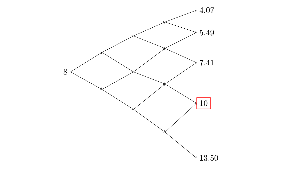
Figure 2.12 4-period flexible binomial tree. The parameters are $S_0=8,K=10,T=1,\sigma=0.3,r=6\%$.

Function 2.7 calculates European option prices using the flexible binomial tree.

Function 2.7: European option pricing on a flexible binomial tree

Download the Jupyter notebook to access the full code.

The flexible binomial tree convergence experiment uses even step counts $n=50,52,\ldots,500$. The calculations include flexible binomial tree and CRR binomial tree prices, along with the absolute errors of the flexible tree prices relative to the Black–Scholes price.

# Calculate flexible tree, CRR tree, and Black-Scholes benchmark prices
flexible_steps = np.arange(50, 501, 2)
flexible_prices = np.array([
    european_flexible_binomial_price(convergence_model, itm_option, replace(settings, n_steps=int(steps)))
    for steps in flexible_steps
])
crr_flexible_prices = np.array([
    european_crr_price(convergence_model, itm_option, replace(settings, n_steps=int(steps)))
    for steps in flexible_steps
])
flexible_bs = black_scholes_formula(
    convergence_model.volatility, itm_option.spot, itm_option.strike,
    itm_option.maturity, convergence_model.rate, itm_option.cp,
)
flexible_errors = np.abs(flexible_prices - flexible_bs)

To plot error convergence, also calculate flexible tree prices at odd step counts. The price plot uses the even step counts from the preceding cell.

# Calculate flexible tree errors including odd step counts for the convergence plot
flexible_error_steps = np.arange(51, 501)
flexible_error_prices = np.array([
    european_flexible_binomial_price(convergence_model, itm_option, replace(settings, n_steps=int(steps)))
    for steps in flexible_error_steps
])
flexible_error_values = np.abs(flexible_error_prices - flexible_bs)

Figure 2.13 shows that the flexible tree prices for the in-the-money put converge to the Black–Scholes price with some local fluctuations. The convergence curve is nevertheless much smoother than that of the CRR tree. Whereas CRR prices oscillate around the Black–Scholes price, the flexible tree consistently underestimates the option price and has larger errors than the CRR tree.

# Figure 2.13: Flexible tree in-the-money European put prices for even step counts
fig, ax = plt.subplots(figsize=(8.0, 5.0))
ax.plot(
    flexible_steps,
    crr_flexible_prices,
    color="black",
    linestyle=":",
    label="CRR price",
)
ax.plot(
    flexible_steps,
    flexible_prices,
    color="red",
    label="Flexible tree price",
)
ax.axhline(
    flexible_bs,
    color="blue",
    linestyle="--",
    label="Black–Scholes price",
)
ax.set_xlabel("Binomial steps $n$")
ax.set_ylabel("European put price")
ax.set_title("Flexible tree in-the-money put price convergence")
ax.legend(frameon=False)
ax.grid(True, alpha=0.25)
fig.tight_layout()
plt.show()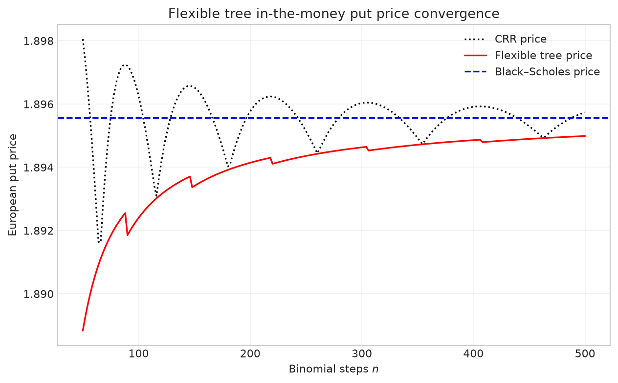

$Figure 2.13 In-the-money European put option prices obtained from flexible binomial trees with varying numbers of steps (even step counts only). The option parameters are $S_0=8,K=10,T=1,\sigma=0.3,r=6\%$.$

Figure 2.13 In-the-money European put option prices obtained from flexible binomial trees with varying numbers of steps (even step counts only). The option parameters are $S_0=8,K=10,T=1,\sigma=0.3,r=6\%$.

Figure 2.14 shows that the flexible binomial tree error converges at a rate of $O(1/n)$.

# Figure 2.14: Flexible tree in-the-money European put error convergence
fig, ax = plt.subplots(figsize=(8.0, 5.0))
ax.loglog(
    flexible_error_steps,
    flexible_error_values,
    color="red",
    linewidth=1.0,
    label="Flexible tree error",
)
ax.loglog(
    flexible_error_steps,
    flexible_error_values[0]
    * (flexible_error_steps[0] / flexible_error_steps),
    "--",
    color="blue",
    label="$1/n$",
)
ax.set_xlabel("Binomial steps $n$")
ax.set_ylabel("Absolute price error")
ax.set_title("Flexible tree in-the-money put error")
ax.legend(frameon=False)
ax.grid(True, which="both", alpha=0.25)
fig.tight_layout()
plt.show()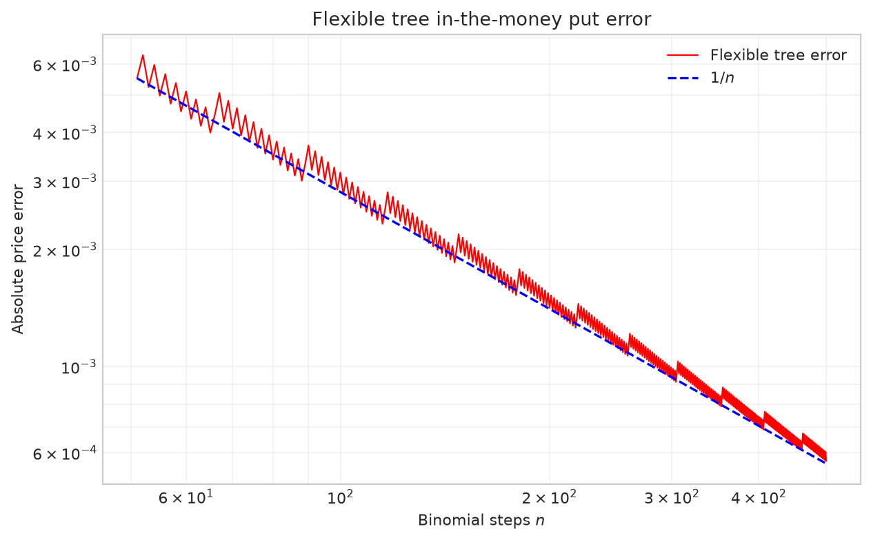

$Figure 2.14 The red solid line shows the pricing errors for an in-the-money European put option on flexible binomial trees with varying numbers of steps $n$. The blue dashed line converges to 0 at a rate of $1/n$. The option parameters are $S_0=8,K=10,T=1,\sigma=0.3,r=6\%$.$

Figure 2.14 The red solid line shows the pricing errors for an in-the-money European put option on flexible binomial trees with varying numbers of steps $n$. The blue dashed line converges to 0 at a rate of $1/n$. The option parameters are $S_0=8,K=10,T=1,\sigma=0.3,r=6\%$.

2.2.2 Richardson Extrapolation

In Figure 2.13, the flexible binomial tree price curve is relatively smooth, allowing extrapolation to cancel the leading error. Combining the flexible binomial tree with Richardson extrapolation can significantly reduce the error in option price estimates (see Chang et al. (2007)). Let $V_n$ and $V_{n/2}$ denote the binomial tree option price estimates using $n$ steps (with an even step count) and $n/2$ steps, respectively. Then

\[ V_n^{RE}=2V_n-V_{n/2}. \tag{2.2.7} \]

Richardson extrapolation uses price estimates at two step counts to cancel the leading error. Let the true price be $V$, and assume that the two step counts being compared have the same leading error coefficient $a$. We can then write

\[\begin{aligned} V_n&=V+\frac{a}{n}+O(n^{-2}),\\ V_{n/2}&=V+\frac{2a}{n}+O(n^{-2}),\\ 2V_n-V_{n/2}&=V+O(n^{-2}). \end{aligned}\]

Substituting these two expansions into equation (2.2.7) cancels the $a/n$ term, leaving an error of $O(n^{-2})$.

For European options, Richardson extrapolation is implemented in Function 2.8.

From Formulas to Code

value_n and value_n_over_2 correspond to the price estimates for $n$ and $n/2$ steps in equation (2.2.7), namely $V_n$ and $V_{n/2}$, respectively; the returned value corresponds to $V_n^{RE}$.

Function 2.8: Richardson extrapolation

Download the Jupyter notebook to access the full code.

The experiment below calculates flexible binomial tree and CRR binomial tree prices, together with their respective Richardson-extrapolated prices, for even step counts $n=50,52,\ldots,500$.

# Calculate base prices for the flexible and CRR trees
richardson_steps = np.arange(50, 501, 2)
flexible_base_prices = np.array([
    european_flexible_binomial_price(convergence_model, itm_option, replace(settings, n_steps=int(steps)))
    for steps in richardson_steps
])
crr_base_prices = np.array([
    european_crr_price(convergence_model, itm_option, replace(settings, n_steps=int(steps)))
    for steps in richardson_steps
])

After the base tree prices have been calculated, the Richardson extrapolation formula is applied to each of the two binomial trees.

# Calculate Richardson extrapolated prices for the flexible and CRR trees
flexible_half_prices = np.array([
    european_flexible_binomial_price(
        convergence_model, itm_option, replace(settings, n_steps=int(steps // 2))
    )
    for steps in richardson_steps
])
crr_half_prices = np.array([
    european_crr_price(
        convergence_model, itm_option, replace(settings, n_steps=int(steps // 2))
    )
    for steps in richardson_steps
])
flexible_re_prices = richardson_extrapolation(
    flexible_base_prices, flexible_half_prices
)
crr_re_prices = richardson_extrapolation(crr_base_prices, crr_half_prices)

Figure 2.15 compares the flexible binomial tree prices with the Richardson-extrapolated prices. The extrapolated prices are closer to the Black–Scholes price.

# Figure 2.15: Flexible tree with Richardson extrapolation for an in-the-money European put
fig, ax = plt.subplots(figsize=(8.0, 5.0))
ax.plot(
    richardson_steps,
    flexible_base_prices,
    color="black",
    linestyle=":",
    label="Flexible tree price",
)
ax.plot(
    richardson_steps,
    flexible_re_prices,
    color="red",
    label="Flexible tree + Richardson extrapolation",
)
ax.axhline(
    flexible_bs,
    color="blue",
    linestyle="--",
    label="Black–Scholes price",
)
ax.set_xlabel("Binomial steps $n$")
ax.set_ylabel("European put price")
ax.set_title("Flexible tree Richardson extrapolation")
ax.legend(frameon=False)
ax.grid(True, alpha=0.25)
fig.tight_layout()
plt.show()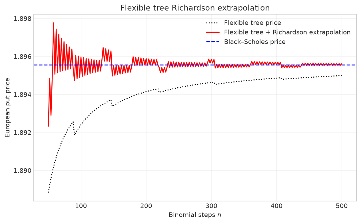

$Figure 2.15 In-the-money European put prices from flexible binomial trees with Richardson extrapolation at varying step counts. The option parameters are $S_0=8,K=10,T=1,\sigma=0.3,r=6\%$.$

Figure 2.15 In-the-money European put prices from flexible binomial trees with Richardson extrapolation at varying step counts. The option parameters are $S_0=8,K=10,T=1,\sigma=0.3,r=6\%$.

It would be tempting to also apply Richardson extrapolation to the CRR binomial tree. However, in the CRR experiment shown in Figure 2.16, the irregular convergence of the CRR tree leads to larger price oscillations after extrapolation, reducing the accuracy of the estimates.

# Figure 2.16: CRR Richardson extrapolation; the changing error coefficient produces oscillations
fig, ax = plt.subplots(figsize=(8.0, 5.0))
ax.plot(
    richardson_steps,
    crr_base_prices,
    color="black",
    linestyle=":",
    label="CRR price",
)
ax.plot(
    richardson_steps,
    crr_re_prices,
    color="red",
    label="CRR + Richardson extrapolation",
)
ax.axhline(
    flexible_bs,
    color="blue",
    linestyle="--",
    label="Black–Scholes price",
)
ax.set_xlabel("Binomial steps $n$")
ax.set_ylabel("European put price")
ax.set_title("CRR Richardson extrapolation")
ax.legend(frameon=False)
ax.grid(True, alpha=0.25)
fig.tight_layout(pad=2.0)
fig.subplots_adjust(left=0.17)
plt.show()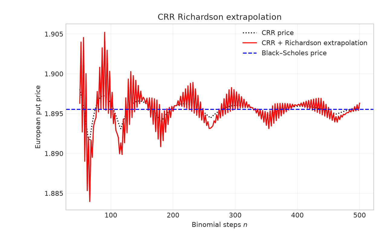

$Figure 2.16 In-the-money European put prices from CRR binomial trees with Richardson extrapolation at varying step counts. The option parameters are $S_0=8,K=10,T=1,\sigma=0.3,r=6\%$.$

Figure 2.16 In-the-money European put prices from CRR binomial trees with Richardson extrapolation at varying step counts. The option parameters are $S_0=8,K=10,T=1,\sigma=0.3,r=6\%$.

2.2.3 American Options

The flexible binomial tree can also be used to price American options; see Function 2.9.

Function 2.9: American option pricing on a flexible binomial tree

Download the Jupyter notebook to access the full code.

We now consider the American version of the put option with parameters $S_0=8,K=10,T=1$ from the preceding example. The experiment uses even step counts $n=50,52,\ldots,500$ to calculate flexible binomial tree prices and Richardson-extrapolated prices, with the Boyle trinomial tree price at $n=20000$ as the numerical benchmark. The Boyle trinomial tree pricing method is discussed in Section 2.4.2.

# American put with the same parameters as the European put
american_put_option = AmericanOption.put(
    spot=itm_option.spot,
    strike=itm_option.strike,
    maturity=itm_option.maturity,
)

# Calculate intermediate results using the parameters and formulas above
flexible_american_prices = np.array([
    american_flexible_binomial_price(
        convergence_model, american_put_option, replace(settings, n_steps=int(steps))
    )
    for steps in richardson_steps
])
flexible_american_half_prices = np.array([
    american_flexible_binomial_price(
        convergence_model, american_put_option, replace(settings, n_steps=int(steps // 2))
    )
    for steps in richardson_steps
])
flexible_american_re_prices = richardson_extrapolation(
    flexible_american_prices, flexible_american_half_prices
)
from quant_option_pricing.trees import (
    american_boyle_trinomial_price as boyle_reference_price,
)
boyle_american_reference = boyle_reference_price(
    convergence_model,
    american_put_option,
    replace(settings, n_steps=20000),
)

pd.Series({
    "Boyle benchmark (20,000 steps)": boyle_american_reference,
})

Boyle benchmark (20,000 steps)    2.103992
dtype: float64

Figure 2.17 shows the flexible binomial tree prices for the American put option in this example and the prices after Richardson extrapolation. The extrapolated curve is closer to the benchmark obtained from a finely discretized tree, illustrating the gain in accuracy from cancelling the leading error.

# Figure 2.17: Flexible tree with Richardson extrapolation for an in-the-money American put
fig, ax = plt.subplots(figsize=(8.0, 5.0))
ax.plot(
    richardson_steps,
    flexible_american_prices,
    color="magenta",
    linestyle=":",
    label="Flexible tree price",
)
ax.plot(
    richardson_steps,
    flexible_american_re_prices,
    color="red",
    label="Flexible tree + Richardson extrapolation",
)
ax.axhline(
    boyle_american_reference,
    color="blue",
    linestyle="--",
    label="Benchmark: Boyle trinomial tree",
)
ax.set_xlabel("Binomial steps $n$")
ax.set_ylabel("American put price")
ax.set_title("American put: flexible tree Richardson extrapolation")
ax.legend(frameon=False)
ax.grid(True, alpha=0.25)
fig.tight_layout()
plt.show()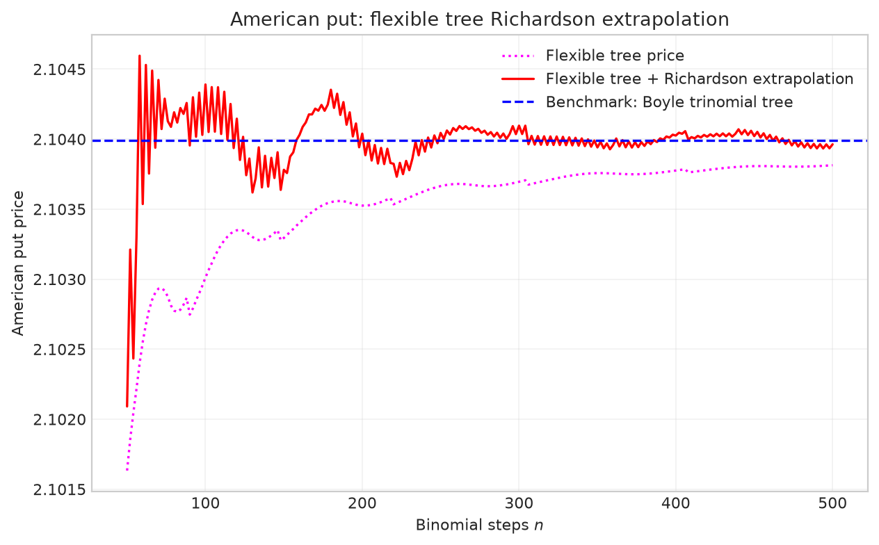

$Figure 2.17 In-the-money American put prices from flexible binomial trees with Richardson extrapolation at varying step counts. The option parameters are $S_0=8,K=10,T=1,\sigma=0.3,r=6\%$.$

Figure 2.17 In-the-money American put prices from flexible binomial trees with Richardson extrapolation at varying step counts. The option parameters are $S_0=8,K=10,T=1,\sigma=0.3,r=6\%$.

2.3 Binomial Black–Scholes Tree for American Option Pricing

To price American options, Broadie and Detemple (1996) proposed calculating the continuation value at the penultimate tree level using the Black–Scholes formula and comparing it with the immediate exercise payoff. This is called the binomial Black–Scholes tree. Smoothing the kink in the terminal payoff reduces the error caused by the relative position of the strike and terminal nodes, discussed in Section 2.1.4. The resulting prices converge more smoothly as the number of steps increases.

Function 2.10 applies this Black–Scholes smoothing to the CRR tree to price American options.

From Formulas to Code

At initialization, stock_prices stores the $n$ stock price nodes at time $T-h$; time_step is the remaining time to maturity $h$ at this level and is passed to black_scholes_formula as the maturity parameter.

values initially stores the Black–Scholes continuation values at these nodes. After an elementwise comparison with the immediate exercise payoffs, it stores the American option values at time $T-h$. The loop then continues backward induction from this level.

Function 2.10: American option pricing with a smoothed CRR binomial tree

Download the Jupyter notebook to access the full code.

The smoothed binomial tree convergence experiment uses even step counts $n=50,52,\ldots,500$.

# Figure 2.18: Calculate ordinary and smoothed CRR price sequences
smooth_steps = np.arange(50, 501, 2)
crr_american_prices = np.array([
    american_crr_price(
        convergence_model, american_put_option, replace(settings, n_steps=int(steps))
    )
    for steps in smooth_steps
])
smoothed_crr_american_prices = np.array([
    smoothed_crr_american_price(
        convergence_model, american_put_option, replace(settings, n_steps=int(steps))
    )
    for steps in smooth_steps
])

Figure 2.18 compares the ordinary CRR tree and the smoothed CRR tree for the in-the-money American put option in this example, with parameters $S_0=8,K=10,T=1,\sigma=0.3,r=6\%$.

The benchmark is the numerical approximation from a Boyle trinomial tree with $n=20000$; the method is discussed in Section 2.4.
Ordinary CRR prices oscillate as the number of steps $n$ increases, just as they do for European options.
The smoothed CRR tree has substantially smaller pricing errors than the ordinary tree, especially for $n>200$.

# Figure 2.18: Ordinary and smoothed CRR prices for an in-the-money American put

fig, ax = plt.subplots(figsize=(8.0, 5.0))
ax.plot(
    smooth_steps,
    crr_american_prices,
    color="black",
    linestyle=":",
    label="CRR price",
)
ax.plot(
    smooth_steps,
    smoothed_crr_american_prices,
    color="red",
    label="Smoothed CRR price",
)
ax.axhline(
    boyle_american_reference,
    color="blue",
    linestyle="--",
    label="Benchmark: Boyle tree, 20,000 steps",
)
ax.set_xlabel("Binomial steps $n$")
ax.set_ylabel("American put price")
ax.set_title("Ordinary and smoothed CRR trees")
ax.legend(frameon=False)
ax.grid(True, alpha=0.25)
fig.tight_layout()
plt.show()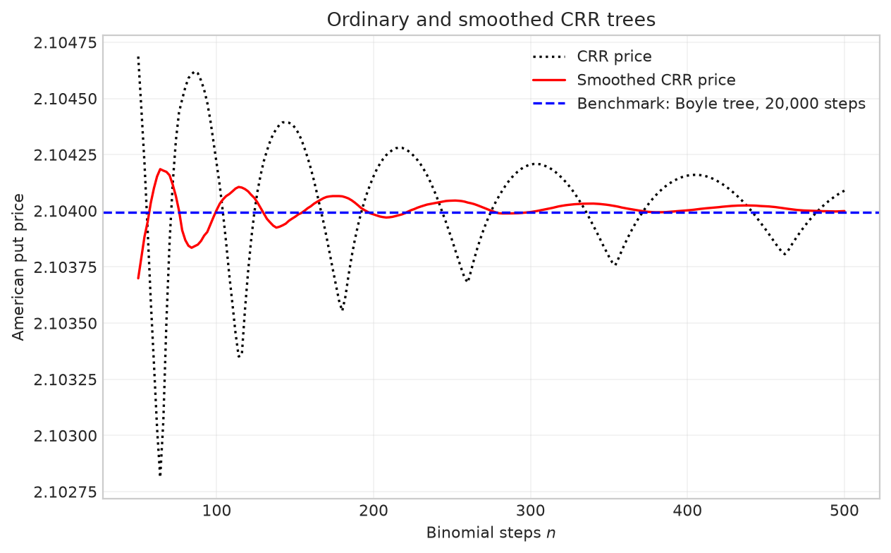

$Figure 2.18 In-the-money American put option prices obtained from smoothed CRR binomial trees with varying numbers of steps (even step counts only). The option parameters are $S_0=8,K=10,T=1,\sigma=0.3,r=6\%$.$

Figure 2.18 In-the-money American put option prices obtained from smoothed CRR binomial trees with varying numbers of steps (even step counts only). The option parameters are $S_0=8,K=10,T=1,\sigma=0.3,r=6\%$.

The binomial Black–Scholes tree can also be combined with the flexible binomial tree; see Function 2.11.

Function 2.11: American option pricing with a smoothed flexible binomial tree

Download the Jupyter notebook to access the full code.

This experiment uses the same parameters and even step counts $n=50,52,\ldots,500$ as the preceding experiment, with smoothing applied only to the flexible binomial tree.

# Figure 2.19: Calculate smoothed flexible tree prices
smoothed_flexible_american_prices = np.array([
    smoothed_flexible_american_price(
        convergence_model, american_put_option, replace(settings, n_steps=int(steps))
    )
    for steps in smooth_steps
])

Figure 2.19 shows that smoothing reduces the flexible binomial tree error. The resulting pricing error is very close to that of the smoothed CRR tree, although the convergence curve still exhibits several jumps.

# Figure 2.19: Smoothed flexible tree prices for an in-the-money American put

fig, ax = plt.subplots(figsize=(8.0, 5.0))
ax.plot(
    smooth_steps,
    smoothed_crr_american_prices,
    color="black",
    label="Smoothed CRR price",
)
ax.plot(
    smooth_steps,
    flexible_american_prices,
    color="magenta",
    linestyle=":",
    label="Flexible tree price",
)
ax.plot(
    smooth_steps,
    smoothed_flexible_american_prices,
    color="red",
    marker="o",
    markersize=2.0,
    label="Smoothed flexible tree price",
)
ax.axhline(
    boyle_american_reference,
    color="blue",
    linestyle="--",
    label="Benchmark: Boyle tree, 20,000 steps",
)
ax.set_xlabel("Binomial steps $n$")
ax.set_ylabel("American put price")
ax.set_title("Smoothed flexible tree")
ax.legend(frameon=False)
ax.grid(True, alpha=0.25)
fig.tight_layout()
plt.show()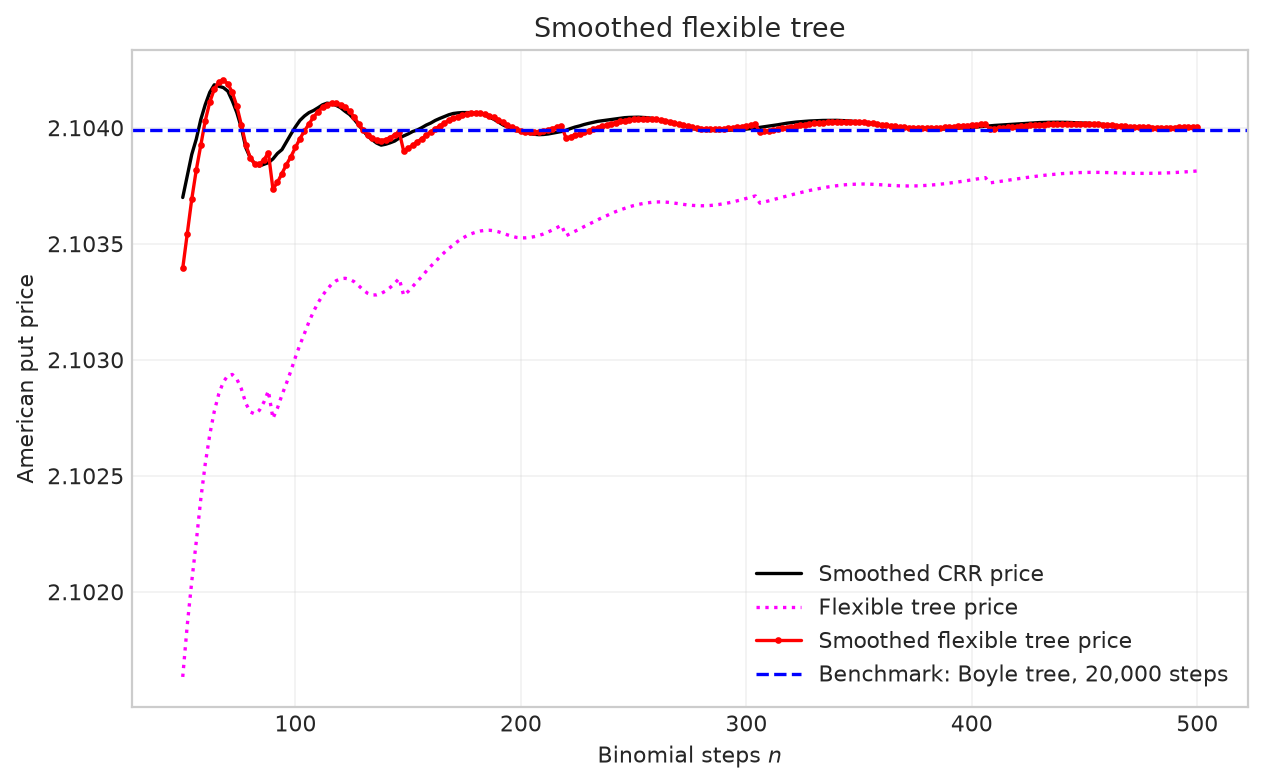

$Figure 2.19 In-the-money American put option prices obtained from smoothed flexible binomial trees with varying numbers of steps (even step counts only). The option parameters are $S_0=8,K=10,T=1,\sigma=0.3,r=6\%$$

Figure 2.19 In-the-money American put option prices obtained from smoothed flexible binomial trees with varying numbers of steps (even step counts only). The option parameters are $S_0=8,K=10,T=1,\sigma=0.3,r=6\%$

The smoothed CRR and smoothed flexible-tree curves nearly coincide. In this example, placing the strike on a terminal node therefore adds little further accuracy once Black–Scholes smoothing has been applied. The two improvements address largely the same source of error: the kink in the terminal put payoff $g(S)=(K-S)^+$.

Strike alignment controls how this kink is sampled by the terminal nodes. Black–Scholes smoothing instead uses the analytical continuation value at the penultimate time $T-h$:

\[ V_{n-1}(S)=\max\left\{(K-S)^+,P_{\mathrm{BS}}(S,K,h)\right\}, \]

where $P_{\mathrm{BS}}(S,K,h)$ is the European put value with remaining maturity $h$. This formula integrates over the final-period stock-price distribution, replacing the two-successor-node approximation to the terminal payoff. Much of the error that strike alignment is intended to reduce has therefore already been removed by smoothing.

2.4 Boyle Trinomial Tree

Boyle (1986) proposed a trinomial tree to improve pricing accuracy. Its three branch probabilities match both the conditional mean and the conditional second moment of the stock price. On a trinomial tree, if the stock price at time $kh$ is $S_k$, the stock price at time $(k+1)h$ can take three values:

With probability $p_u$, it rises to $uS_k$;
With probability $p_d$, it falls to $dS_k$;
With probability $p_m=1-p_u-p_d$, it changes to $mS_k$,

where $u>m>d$. A recombining trinomial tree like the one in Figure 2.20 requires

\[ ud=m^2. \tag{2.4.1} \]

For the same number of steps $n$, a binomial tree has $n+1$ terminal nodes and a trinomial tree has $2n+1$. At each node, backward induction requires a discounted expectation over two successors for the binomial tree and three for the trinomial tree. The trinomial tree therefore requires more computation.

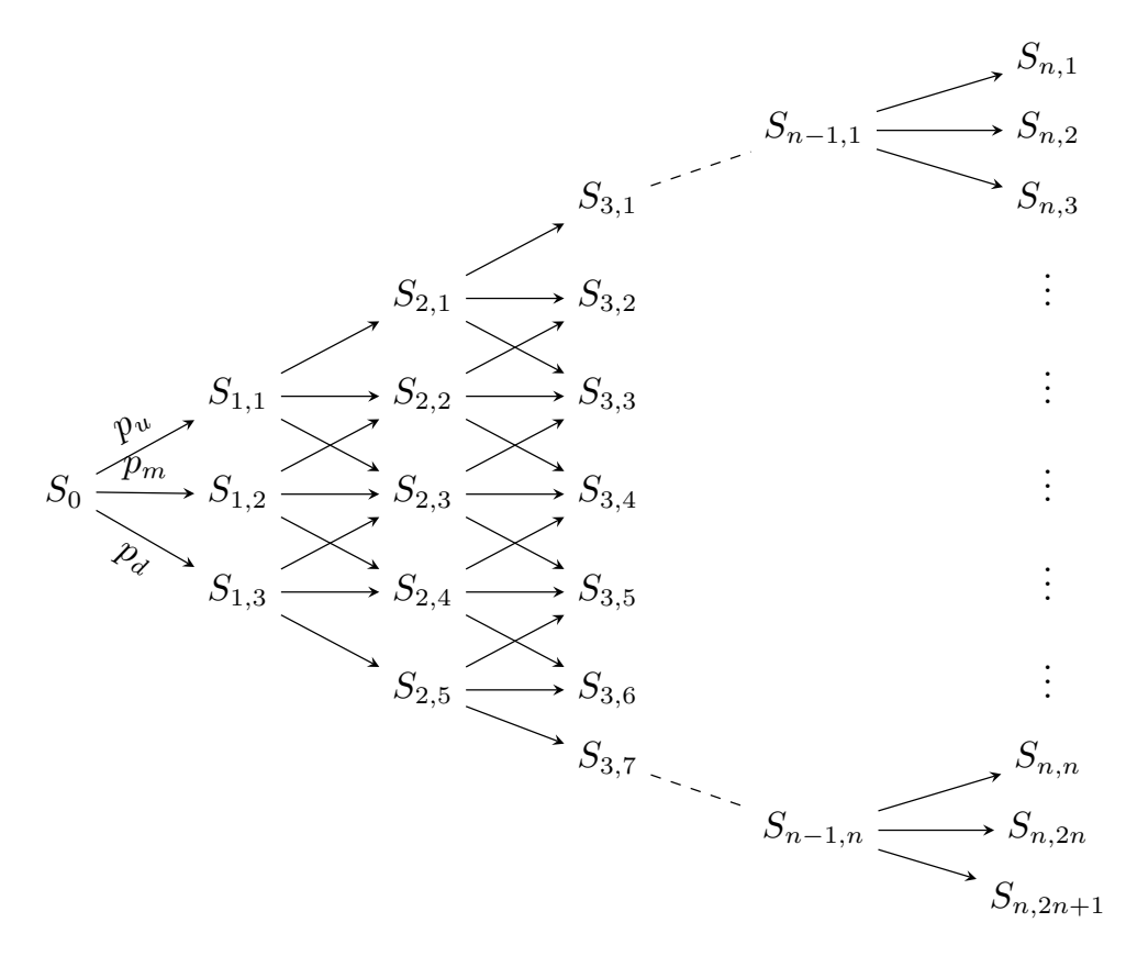
Nodes of an n-period Boyle trinomial tree.

Figure 2.20 Nodes of an $n$-period Boyle trinomial tree.

On the trinomial tree shown in Figure 2.20, if an upward branch represents a decline in stock price, Table 2.5 gives the nodes at time $kh$.

Node	Node value
$S_{k,1}$	$S_0 d^k u^0$
$S_{k,2}$	$S_0 d^{k-1} u^0$
$S_{k,3}$	$S_0 d^{k-1} u^1$
$S_{k,4}$	$S_0 d^{k-2} u^1$
$S_{k,5}$	$S_0 d^{k-2} u^2$
$\vdots$	$\vdots$
$S_{k,2k-1}$	$S_0 d^1 u^{k-1}$
$S_{k,2k}$	$S_0 d^0 u^{k-1}$
$S_{k,2k+1}$	$S_0 d^0 u^k$

Table 2.5 Stock prices at the trinomial tree nodes at time $kh$.

First calculate the parameters for one step of the trinomial tree using these formulas.

Given the stock price at time $kh$, denoted by $S_k$, the probabilities $p_u,p_d,p_m$ correspond to next-period stock prices of $uS_k,dS_k,mS_k$, respectively. Thus, the conditional mean is the probability-weighted average of these three possible stock prices; the conditional second moment is obtained by squaring each possible stock price and weighting it by the same probability. Matching these two conditional moments to the one-step conditional moments of risk-neutral geometric Brownian motion requires the Boyle trinomial tree parameters $u,d,p_u,p_d$ to satisfy the following equations:

\[ p_uuS_k+p_ddS_k+(1-p_u-p_d)mS_k=S_kM \tag{2.4.2} \]

\[ p_uu^2S_k^2+p_dd^2S_k^2+(1-p_u-p_d)m^2S_k^2=S_k^2M^2\Psi \tag{2.4.3} \]

\[ ud=m^2. \tag{2.4.4} \]

where

\[ M=e^{rh},\qquad \Psi=e^{\sigma^2h}. \tag{2.4.5} \]

In equation (2.4.2), the left-hand side is the tree’s conditional mean, while the right-hand side $S_kM$ is the conditional mean of risk-neutral geometric Brownian motion from equation (2.1.7). Similarly, equation (2.4.3) equates the tree’s conditional second moment to $S_k^2M^2\Psi$, the conditional second moment from equation (2.1.8). Since conditional variance equals the conditional second moment minus the square of the conditional mean, the conditional variance of the next-period stock price is $S_k^2M^2(\Psi-1)$.

For three given node positions, the upward, middle, and downward probabilities must sum to 1 and match the conditional mean and conditional second moment. Set the middle factor $m=1$, meaning that the middle branch leaves the stock price unchanged, and combine this with the recombining condition $ud=1$. Solving equations (2.4.2)–(2.4.4) under these conditions gives

\[ m=1, \qquad p_u=\frac{md-M(m+d)+M^2\Psi}{(u-d)(u-m)}, \tag{2.4.6} \]

\[ p_d=\frac{um-M(u+m)+M^2\Psi}{(u-d)(m-d)}, \qquad p_m=1-p_u-p_d. \tag{2.4.7} \]

Equations (2.4.2)–(2.4.4) allow several choices of $u$ and $d$. Using the CRR binomial tree choice $u=e^{\sigma\sqrt h}$ leads to $p_m<0$ in many cases. To avoid this problem, Boyle (1986）introduces an additional parameter $\lambda$ so that

\[ u=e^{\lambda\sigma\sqrt h},\qquad d=e^{-\lambda\sigma\sqrt h}, \tag{2.4.8} \]

and recommends using $\lambda=1.2$.

The parameter $\lambda$ controls the distance of the upper and lower nodes from the middle node: increasing $\lambda$ increases the spacing between the upper and lower stock prices. The three branch probabilities are then recalculated to preserve the specified conditional mean and conditional variance. The spacing must also be chosen so that all three probabilities lie in $[0,1]$. The flexible binomial tree introduced in Section 2.2 also uses the symbol $\lambda$, but there it tilts the entire binomial tree grid; here it adjusts the spacing between the trinomial tree branches.

Function 2.12 generates a Boyle trinomial tree under these conditions and can be used to price both European and American options.

From Formulas to Code

growth corresponds to $M=e^{rh}$, variance_growth corresponds to $\Psi=e^{\sigma^2h}$, and middle corresponds to $m=1$; spacing corresponds to the spacing parameter $\lambda$ in equation (2.4.8).

p_up and p_down correspond to $p_u$ and $p_d$. up_exponents and down_exponents store the exponents of $u$ and $d$ in Table 2.5; multiplying the returned power arrays elementwise and scaling the result by $S_0$ gives the $2n+1$ terminal stock prices in ascending order.

Function 2.12: Boyle trinomial tree parameters

Download the Jupyter notebook to access the full code.

Using the chapter’s default parameters $T=0.5,\sigma=0.2,r=6\%,n=100$ and $\lambda=1.2$, call Function 2.12 to calculate the Boyle tree’s upward and downward probabilities.

# Use Function 2.12 to obtain Boyle upward and downward probabilities
_, _, boyle_up_probability, boyle_down_probability, _ = boyle_tree_parameters(
    model, option.maturity, settings.n_steps, settings.trinomial_lambda
)

Function 2.12 returns $p_u$ and $p_d$; equation (2.4.7) then gives the middle branch probability as $p_m=1-p_u-p_d$. The three probabilities are listed below.

# Display risk-neutral probabilities for the three Boyle branches
boyle_middle_probability = 1.0 - boyle_up_probability - boyle_down_probability
pd.Series(
    {
        "p_d": boyle_down_probability,
        "p_m": boyle_middle_probability,
        "p_u": boyle_up_probability,
    }
)

p_d    0.341572
p_m    0.305073
p_u    0.353355
dtype: float64

2.4.1 European Options

European option pricing on the Boyle trinomial tree begins by calculating the $2n+1$ terminal payoffs, then proceeds backward. At each node, the value is the discounted risk-neutral expectation of the values at its three adjacent successor nodes. Function 2.13 implements this recursion.

From Formulas to Code

p_middle corresponds to $p_m=1-p_u-p_d$. When working backward from level $i$ to level $i-1$, values[:2*i-1], values[1:2*i], and values[2:2*i+1] provide the downward, middle, and upward successor values for each node, respectively. After weighting and discounting, the number of nodes decreases from $2i+1$ to $2i-1$.

Function 2.13: European option pricing on a Boyle trinomial tree

Download the Jupyter notebook to access the full code.

The Boyle trinomial tree convergence experiment uses the at-the-money option parameters $S_0=K=10,T=1,\sigma=0.3,r=6\%$ and even step counts $n=50,52,\ldots,500$.

The calculation uses these at-the-money parameters and also retains the CRR binomial tree prices and the Black–Scholes benchmark price.

# Calculate intermediate results using the parameters and formulas above
trinomial_steps = np.arange(50, 501, 2)
boyle_atm_prices = np.array(
    [
        european_boyle_trinomial_price(
            convergence_model,
            atm_option,
            replace(settings, n_steps=int(steps)),
        )
        for steps in trinomial_steps
    ]
)
crr_atm_trinomial_prices = np.array(
    [
        european_crr_price(
            convergence_model,
            atm_option,
            replace(settings, n_steps=int(steps)),
        )
        for steps in trinomial_steps
    ]
)
boyle_atm_bs = black_scholes_formula(
    convergence_model.volatility,
    atm_option.spot,
    atm_option.strike,
    atm_option.maturity,
    convergence_model.rate,
    atm_option.cp,
)
crr_atm_errors = np.abs(crr_atm_trinomial_prices - boyle_atm_bs)
boyle_atm_errors = np.abs(boyle_atm_prices - boyle_atm_bs)

Figure 2.21 compares prices from the two trees at even step counts, using the at-the-money European put parameters $S_0=K=10,T=1,\sigma=0.3,r=6\%$. With these parameters, the Boyle tree performs particularly well: its pricing error at $n=50$ is smaller than the CRR error at $n=500$. Its convergence is also smooth when only even step counts $n$ are used.

# Figure 2.21: Boyle at-the-money European put prices, S0=K=10, T=1, sigma=0.3, r=6%
fig, ax = plt.subplots(figsize=(8.0, 5.0))
ax.plot(
    trinomial_steps,
    crr_atm_trinomial_prices,
    color="black",
    linestyle=":",
    label="CRR price: even n",
)
ax.plot(
    trinomial_steps,
    boyle_atm_prices,
    color="red",
    label="Boyle tree: even n",
)
ax.axhline(
    boyle_atm_bs,
    color="blue",
    linestyle="--",
    label="Black–Scholes price",
)
ax.set_xlabel("Trinomial steps $n$")
ax.set_ylabel("European put price")
ax.set_title("Boyle at-the-money put price convergence")
ax.legend(frameon=False)
ax.grid(True, alpha=0.25)
fig.tight_layout()
plt.show()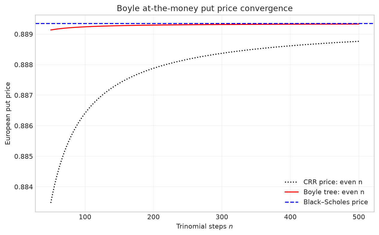

$Figure 2.21 At-the-money European put option prices from the Boyle trinomial tree. The parameters are $S_0=K=10,T=1,\sigma=0.3,r=6\%$.$

Figure 2.21 At-the-money European put option prices from the Boyle trinomial tree. The parameters are $S_0=K=10,T=1,\sigma=0.3,r=6\%$.

Figure 2.22 shows that the Boyle trinomial tree also converges at a rate of $1/n$.

# Figure 2.22: Boyle at-the-money European put errors and the 1/n convergence rate
fig, ax = plt.subplots(figsize=(7.5, 4.2))
ax.loglog(
    trinomial_steps,
    crr_atm_errors,
    "k--",
    label="CRR error",
)
ax.loglog(
    trinomial_steps,
    boyle_atm_errors,
    "r-",
    label="Boyle error",
)
ax.loglog(
    trinomial_steps,
    boyle_atm_errors[0] * (trinomial_steps[0] / trinomial_steps),
    "b--",
    label="$1/n$",
)
ax.set_xlabel("Trinomial steps $n$")
ax.set_ylabel("Absolute price error")
ax.set_title("Boyle at-the-money put error")
ax.legend(frameon=False)
ax.grid(True, which="both", alpha=0.25)
fig.tight_layout()
plt.show()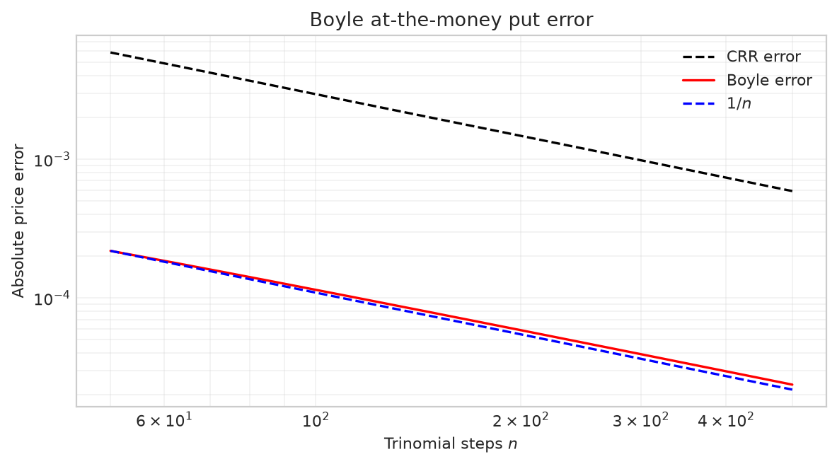

$Figure 2.22 The red solid line shows the pricing errors for an at-the-money European put option on Boyle trinomial trees with varying numbers of steps $n$. The blue dashed line converges to 0 at a rate of $1/n$. The option parameters are $S_0=K=10,T=1,\sigma=0.3,r=6\%$.$

Figure 2.22 The red solid line shows the pricing errors for an at-the-money European put option on Boyle trinomial trees with varying numbers of steps $n$. The blue dashed line converges to 0 at a rate of $1/n$. The option parameters are $S_0=K=10,T=1,\sigma=0.3,r=6\%$.

We next consider an in-the-money option with $S_0=8,K=10,T=1,\sigma=0.3,r=6\%$, using the same grid of even step counts as above. Boyle trinomial and CRR binomial tree prices are calculated and compared against the Black–Scholes benchmark.

# Calculate intermediate results using the parameters and formulas above
boyle_itm_prices = np.array(
    [
        european_boyle_trinomial_price(
            convergence_model,
            itm_option,
            replace(settings, n_steps=int(steps)),
        )
        for steps in trinomial_steps
    ]
)
crr_itm_trinomial_prices = np.array(
    [
        european_crr_price(
            convergence_model,
            itm_option,
            replace(settings, n_steps=int(steps)),
        )
        for steps in trinomial_steps
    ]
)
boyle_itm_bs = black_scholes_formula(
    convergence_model.volatility,
    itm_option.spot,
    itm_option.strike,
    itm_option.maturity,
    convergence_model.rate,
    itm_option.cp,
)
boyle_itm_errors = np.abs(boyle_itm_prices - boyle_itm_bs)
american_trinomial_steps = np.arange(50, 501, 2)

Figure 2.23 shows that both Boyle and CRR prices oscillate around the Black–Scholes price. The Boyle prices oscillate over a narrower range, particularly when $n$ is small and the CRR binomial tree error is large.

# Figure 2.23: Boyle in-the-money European put prices, S0=8, K=10, T=1, sigma=0.3, r=6%
fig, ax = plt.subplots(figsize=(8.0, 5.0))
ax.plot(
    trinomial_steps,
    crr_itm_trinomial_prices,
    color="black",
    linestyle=":",
    label="CRR price: even n",
)
ax.plot(
    trinomial_steps,
    boyle_itm_prices,
    color="red",
    label="Boyle price: even n",
)
ax.axhline(
    boyle_itm_bs,
    color="blue",
    linestyle="--",
    label="Black–Scholes price",
)
ax.set_xlabel("Trinomial steps $n$")
ax.set_ylabel("European put price")
ax.set_title("Boyle in-the-money put price convergence")
ax.legend(frameon=False)
ax.grid(True, alpha=0.25)
fig.tight_layout()
plt.show()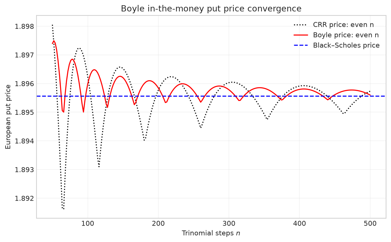

$Figure 2.23 In-the-money European put option prices from the Boyle trinomial tree. The parameters are $S_0=8,K=10,T=1,\sigma=0.3,r=6\%$.$

Figure 2.23 In-the-money European put option prices from the Boyle trinomial tree. The parameters are $S_0=8,K=10,T=1,\sigma=0.3,r=6\%$.

Figure 2.24 shows that the Boyle trinomial tree convergence rate remains $1/n$, with error fluctuations similar to those of the CRR binomial tree.

# Figure 2.24: Boyle in-the-money European put errors; narrower oscillations than CRR with fluctuations in error convergence
fig, ax = plt.subplots(figsize=(7.5, 4.2))
ax.loglog(
    trinomial_steps,
    boyle_itm_errors,
    "r-",
    marker=".",
    markersize=4,
    label="Boyle error",
)
ax.loglog(
    trinomial_steps,
    boyle_itm_errors[0] * (trinomial_steps[0] / trinomial_steps),
    "b--",
    label="$1/n$",
)
ax.set_xlabel("Trinomial steps $n$")
ax.set_ylabel("Absolute price error")
ax.set_title("Boyle in-the-money put error")
ax.legend(frameon=False)
ax.grid(True, which="both", alpha=0.25)
fig.tight_layout()
plt.show()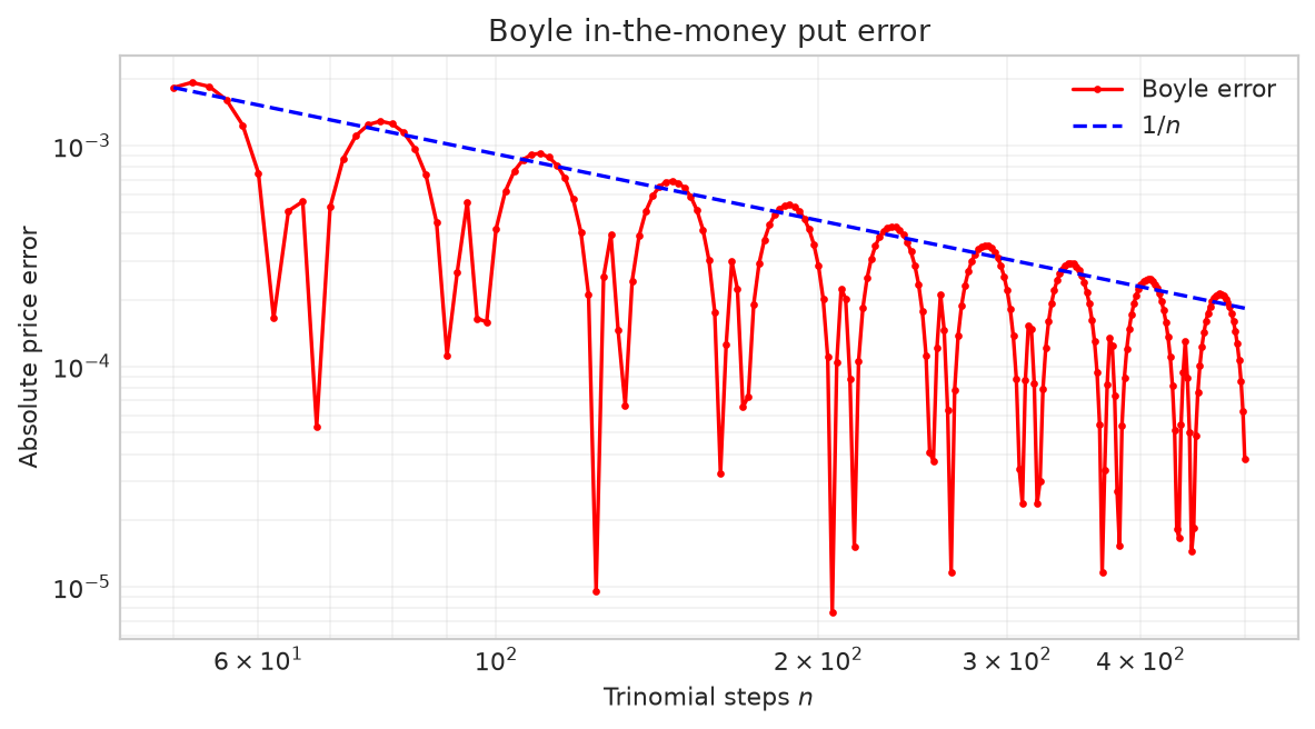

$Figure 2.24 The red solid line shows the pricing errors for an in-the-money European put option on Boyle trinomial trees with varying numbers of steps $n$. The blue dashed line converges to 0 at a rate of $1/n$. The option parameters are $S_0=8,K=10,T=1,\sigma=0.3,r=6\%$.$

Figure 2.24 The red solid line shows the pricing errors for an in-the-money European put option on Boyle trinomial trees with varying numbers of steps $n$. The blue dashed line converges to 0 at a rate of $1/n$. The option parameters are $S_0=8,K=10,T=1,\sigma=0.3,r=6\%$.

2.4.2 American Options

The Boyle trinomial tree can also be used to price American options; see Function 2.14. At each backward step, compare the continuation value from the three successor nodes with the immediate exercise payoff at the current node.

Function 2.14: American option pricing on a Boyle trinomial tree

Download the Jupyter notebook to access the full code.

With $S_0=8,K=10,T=1,\sigma=0.3,r=6\%$ and even step counts $n=50,52,\ldots,500$, the Boyle trinomial tree gives American put option prices. The same method with $n=20000$ provides the numerical benchmark.

# Calculate intermediate results using the parameters and formulas above
boyle_american_prices = np.array([
    american_boyle_trinomial_price(
        convergence_model, american_put_option, replace(settings, n_steps=int(steps))
    )
    for steps in american_trinomial_steps
])
boyle_american_reference = american_boyle_trinomial_price(
    convergence_model,
    american_put_option,
    replace(settings, n_steps=settings.reference_steps),
)
boyle_american_errors = np.abs(
    boyle_american_prices - boyle_american_reference
)

Figure 2.25 shows that the Boyle trinomial tree has smaller errors than the CRR binomial tree.

# Figure 2.25: Boyle prices for an in-the-money American put
fig, ax = plt.subplots(figsize=(8.0, 5.0))
ax.plot(
    american_trinomial_steps,
    crr_american_prices,
    color="black",
    linestyle=":",
    label="CRR price",
)
ax.plot(
    american_trinomial_steps,
    boyle_american_prices,
    color="red",
    label="Boyle price",
)
ax.axhline(
    boyle_american_reference,
    color="blue",
    linestyle="--",
    label="Benchmark: Boyle tree, 20,000 steps",
)
ax.set_xlabel("Trinomial steps $n$")
ax.set_ylabel("American put price")
ax.set_title("Boyle American put prices")
ax.legend(frameon=False)
ax.grid(True, alpha=0.25)
fig.tight_layout(pad=2.0)
plt.show()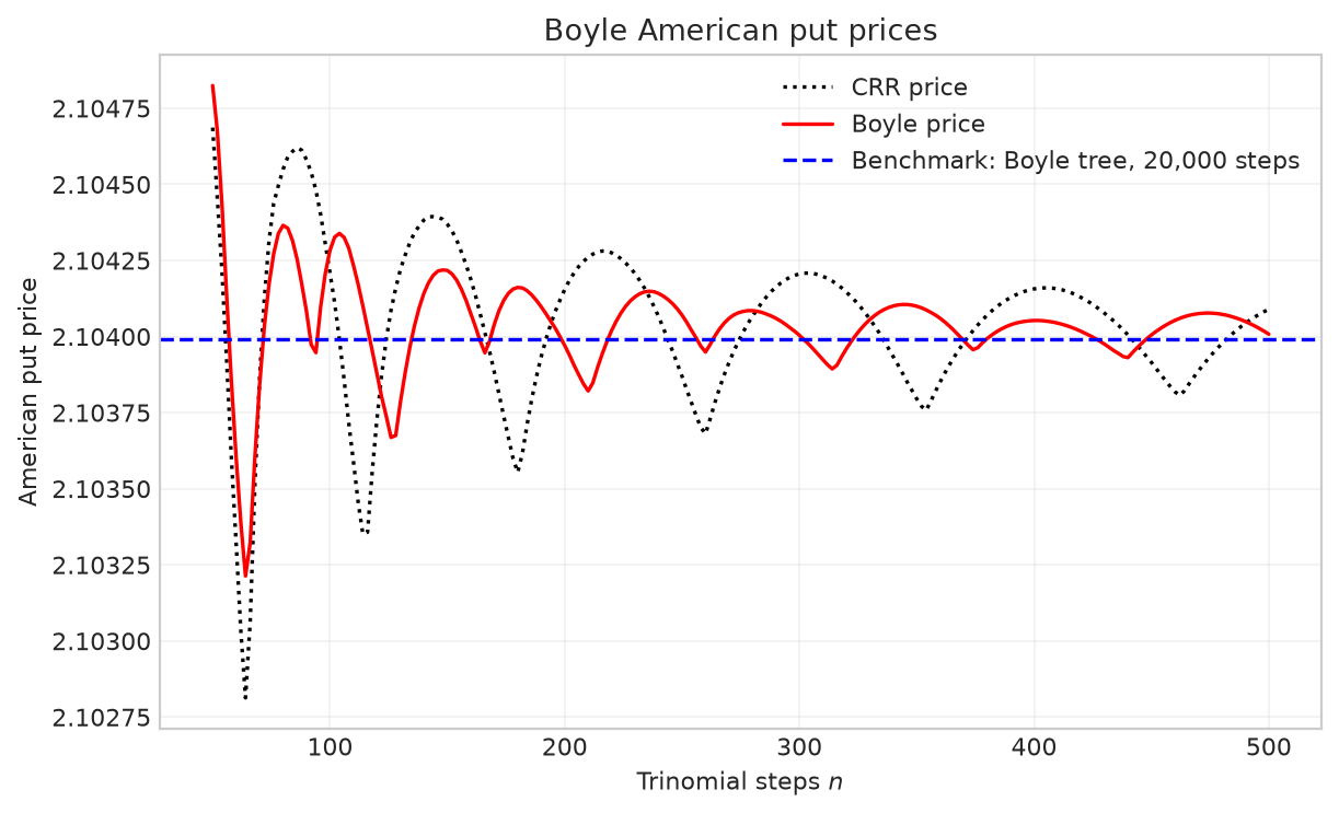

$Figure 2.25 In-the-money American put option prices obtained from Boyle trinomial trees with varying numbers of steps (even $n$ only). The option parameters are $S_0=8,K=10,T=1,\sigma=0.3,r=6\%$.$

Figure 2.25 In-the-money American put option prices obtained from Boyle trinomial trees with varying numbers of steps (even $n$ only). The option parameters are $S_0=8,K=10,T=1,\sigma=0.3,r=6\%$.

The Boyle trinomial tree can also be combined with the Black–Scholes tree method to price American options and produce smoother convergence of option prices. At the penultimate level, the Black–Scholes formula gives the continuation value, which is compared with the immediate exercise payoff. The American option recursion then proceeds backward through the earlier levels. See Function 2.15.

From Formulas to Code

At initialization, down_values[2:] and up_values[:-2] generate the $2n-1$ stock price nodes at time $T-h$, which are stored in stock_prices. At each of these nodes, the remaining time to maturity is time_step, namely $h$; after smoothing and comparison with the immediate exercise payoffs, values stores the American option values at this level.

Function 2.15: American option pricing on a smoothed Boyle trinomial tree

Download the Jupyter notebook to access the full code.

The next cell uses the parameters and even step counts from the preceding experiment to calculate smoothed Boyle trinomial tree prices. These are compared with ordinary Boyle trinomial tree prices and the same benchmark obtained from a finely discretized tree.

# Calculate intermediate results using the parameters and formulas above
smoothed_boyle_american_prices = np.array(
    [
        smoothed_boyle_trinomial_price(
            convergence_model,
            american_put_option,
            replace(settings, n_steps=int(steps)),
        )
        for steps in american_trinomial_steps
    ]
)

Figure 2.26 shows that the smoothed Boyle trinomial tree produces smoother convergence and smaller pricing errors.

# Figure 2.26: Boyle prices for an in-the-money American put
fig, ax = plt.subplots(figsize=(8.0, 5.0))
ax.plot(
    american_trinomial_steps,
    boyle_american_prices,
    color="red",
    label="Boyle price",
)
ax.plot(
    american_trinomial_steps,
    smoothed_boyle_american_prices,
    color="black",
    linestyle=":",
    label="Smoothed Boyle price",
)
ax.axhline(
    boyle_american_reference,
    color="blue",
    linestyle="--",
    label="Benchmark: Boyle tree, 20,000 steps",
)
ax.set_xlabel("Trinomial steps $n$")
ax.set_ylabel("American put price")
ax.set_title("Boyle American put prices")
ax.legend(frameon=False)
ax.grid(True, alpha=0.25)
fig.tight_layout(pad=2.0)
fig.subplots_adjust(left=0.17)
plt.show()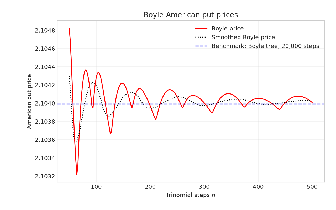

$Figure 2.26 In-the-money American put option prices obtained from smoothed Boyle trinomial trees with varying numbers of steps (even $n$ only). The option parameters are $S_0=8,K=10,T=1,\sigma=0.3,r=6\%$.$

Figure 2.26 In-the-money American put option prices obtained from smoothed Boyle trinomial trees with varying numbers of steps (even $n$ only). The option parameters are $S_0=8,K=10,T=1,\sigma=0.3,r=6\%$.

References

Cox, J. C., Ross, S. A., & Rubinstein, M. (1979). “Option Pricing: A Simplified Approach.” Journal of Financial Economics, 7(3), 229–263.
Higham, D. J. (2002). “Nine Ways to Implement the Binomial Method for Option Valuation in MATLAB.” SIAM Review, 44(4), 661–677.
Hull, J. (2014). Options, Futures, and Other Derivatives (9th edition). Pearson.
Pelsser, A., & Vorst, T. C. F. (1994). “The Binomial Model and the Greeks.” The Journal of Derivatives, 1(3), 45–49.
Diener, F., & Diener, M. (2004). “Asymptotics of the Price Oscillations of a European Call Option in a Tree Model.” Mathematical Finance, 14(2), 271–293.
Broadie, M., & Detemple, J. (1996). “American Option Valuation: New Bounds, Approximations, and a Comparison of Existing Methods.” The Review of Financial Studies, 9(4), 1211–1250.
Leisen, D. P., & Reimer, M. (1996). “Binomial Models for Option Valuation—Examining and Improving Convergence.” Applied Mathematical Finance, 3, 319–346.
Tian, Y. (1993). “A Modified Lattice Approach to Option Pricing.” Journal of Futures Markets, 13, 563–577.
Tian, Y. (1999). “A Flexible Binomial Option Pricing Model.” The Journal of Futures Markets, 19, 817–843.
Chung, S. L., & Shih, P. T. (2007). “Generalized Cox-Ross-Rubinstein Binomial Model.” Management Science, 53, 508–520.
Boyle, P. (1986). “Option Valuation Using a Three-Jump Process.” International Options Journal, 3, 7–12.
Kamrad, B., & Ritchken, P. (1991). “Multinomial Approximating Models for Options with k State Variables.” Management Science, 37(12), 1640–1652.
Joshi, M. (2009). “The Convergence of Binomial Trees for Pricing the American Put.” The Journal of Risk, 11(4), 87–108.
Chan, J. H., Joshi, M., Tang, R., & Yang, C. (2009). “Trinomial or Binomial: Accelerating American Put Option Price on Trees.” The Journal of Futures Markets, 29(9), 826–839.
Chang, C.-C., Chung, S.-L., & Stapleton, R. (2007). “Richardson Extrapolation Techniques for the Pricing of American-Style Options.” Journal of Futures Markets, 27, 791–817.

	\(S_T<K\)	\(S_T\geq K\)
Portfolio 1	\(K\)	\((S_T-K)+K=S_T\)
Portfolio 2	\(S_T\)	\(S_T\)

Node	Node value
\(S_{k,1}\)	\(S_0 d^k u^0\)
\(S_{k,2}\)	\(S_0 d^{k-1} u^0\)
\(S_{k,3}\)	\(S_0 d^{k-1} u^1\)
\(S_{k,4}\)	\(S_0 d^{k-2} u^1\)
\(S_{k,5}\)	\(S_0 d^{k-2} u^2\)
\(\vdots\)	\(\vdots\)
\(S_{k,2k-1}\)	\(S_0 d^1 u^{k-1}\)
\(S_{k,2k}\)	\(S_0 d^0 u^{k-1}\)
\(S_{k,2k+1}\)	\(S_0 d^0 u^k\)

2.1 Cox-Ross-Rubinstein (CRR) Binomial Tree

2.1.1 European Options

2.1.2 \(\Delta\) and \(\Gamma\) Estimation

2.1.2.1 Hull’s Method

2.1.2.2 Extended Binomial Tree

2.1.3 American Options

2.1.4 Convergence Properties of the CRR Binomial Tree

2.2 Flexible Binomial Tree

2.2.1 European Options

2.2.2 Richardson Extrapolation

2.2.3 American Options

2.3 Binomial Black–Scholes Tree for American Option Pricing

2.4 Boyle Trinomial Tree

2.4.1 European Options

2.4.2 American Options

References