# Import the numerical, statistical, and plotting libraries used in this section
import sys
from pathlib import Path

import matplotlib.pyplot as plt
import numpy as np
import pandas as pd
import yfinance as yf
from scipy.integrate import quad
from scipy.stats import kurtosis, norm, poisson, skew

project_root = Path.cwd()
while not (project_root / "src").exists() and project_root != project_root.parent:
    project_root = project_root.parent
sys.path.insert(0, str(project_root / "src"))

plt.style.use("seaborn-v0_8-whitegrid")
plt.rcParams["font.family"] = "sans-serif"
plt.rcParams["font.sans-serif"] = [
    "Microsoft YaHei", "PingFang SC", "Noto Sans CJK SC",
    "WenQuanYi Micro Hei", "SimHei", "DejaVu Sans",
]
plt.rcParams["axes.unicode_minus"] = False
np.set_printoptions(precision=6, suppress=True)
pd.set_option("display.precision", 6)Chapter 1: Stochastic Processes and Risk-Neutral Pricing
In this chapter we begin with option payoffs and introduce Brownian motion, geometric Brownian motion, Merton jump diffusion, Variance Gamma, and Normal Inverse Gaussian models. We then use risk-neutral pricing to derive the Black–Scholes formula and introduce Greeks and implied volatility. We explain how these models describe price changes, calculate option prices from model parameters, and solve for implied volatility from market option prices.
1.1 Introduction to Options
An option is a financial derivative whose value depends on an underlying asset, such as a commodity, stock, currency, interest rate, or index. The buyer pays a premium for the right, but not the obligation, to trade under agreed terms. The seller receives the premium and must fulfil the contract when the buyer exercises the option.
We first distinguish three aspects of an option: calls and puts differ in their payoffs; European, American, and Bermudan options differ in when they can be exercised; Asian, spread, and basket options differ in the asset prices used to determine their payoffs.
Call Options and Put Options
A call option gives the buyer the right to buy the underlying asset at the strike price, typically to express a view that prices will rise or to lock in a future purchase price. For example, if the strike price \(K=100\) and the underlying price at maturity is \(S_T=120\), the buyer can buy an asset worth 120 for 100, receiving a payoff of 20 at maturity; if \(S_T=80\), the buyer will not exercise at 100, and the payoff is 0. The payoff of a European call option at maturity \(T\) is
\[g_C(S_T) = \max(S_T-K,0) = (S_T-K)^+\tag{1.1.1}.\]
A put option gives the buyer the right to sell the underlying asset at the strike price, typically to express a view that prices will fall or to provide protection for an existing position, much like insurance. For example, if \(K=100\) and \(S_T=80\), the buyer can sell an asset worth 80 for 100, receiving a payoff of 20 at maturity; if \(S_T=120\), selling at 100 offers no benefit, and the payoff is 0. The payoff of a European put option is
\[g_P(S_T) = \max(K-S_T,0) = (K-S_T)^+\tag{1.1.2}.\]
Equations (1.1.1) and (1.1.2) give the payoffs at maturity. Here \(S_T\) is the underlying asset price at maturity and \(K\) is the strike price. These payoffs exclude the premium paid initially by the buyer. Ignoring the time value of the premium, the buyer’s net profit or loss at maturity is the payoff minus the premium \(p\). If the premium paid at time 0 is carried forward to maturity at the risk-free rate \(r\), the net profit or loss is \(g(S_T)-pe^{rT}\). The seller’s net profit or loss using the same treatment of interest is the opposite.
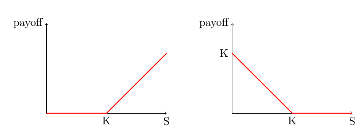
Figure 1.1 Payoff functions of European call (left) and put (right) options at maturity.
Exercise Times: European, American, and Bermudan
European, American, and Bermudan options differ in when the buyer may exercise them: European options can be exercised only at maturity \(T\), American options at any time before expiry, and Bermudan options fall between the two, allowing exercise at predetermined times \(0<T_1<T_2<\cdots<T_M\leq T\). The right to exercise early affects the option’s value. Pricing American and Bermudan options therefore requires considering the asset prices and exercise decisions at each permitted exercise time, as well as the asset price \(S_T\) at maturity.
Path Dependent Options
The payoff of an Asian option depends on the average asset price over a period, rather than the price at a single time. If \(A(T)\) is the continuous or discrete average price over \([0,T]\), the payoff of an Asian call option is \([A(T)-K]^+\), and the corresponding put payoff can be written as \([K-A(T)]^+\). For example, when \(K=100\) and the average price is \(A(T)=105\), the call payoff is 5, even if the price on the maturity date is below 100. Averaging prices smooths short-term fluctuations, making these options less sensitive to single-day price shocks near maturity; they are also often used to reduce the impact of price manipulation at settlement.
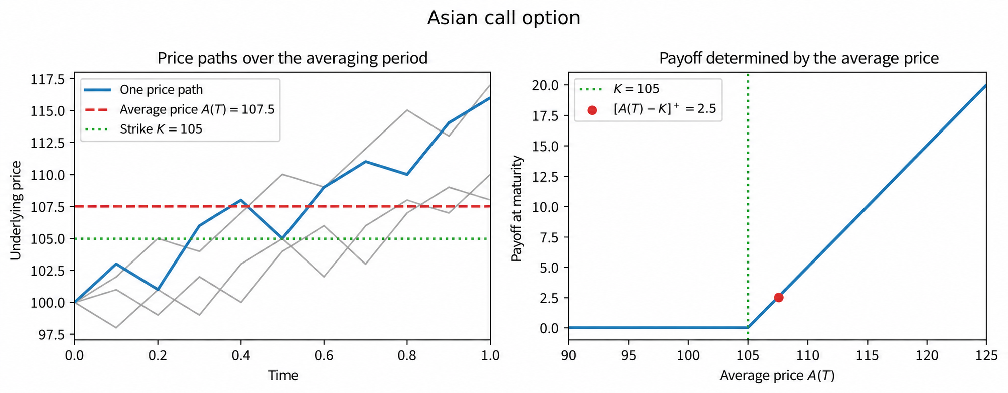
Figure 1.1a Schematic of an Asian call option: the payoff is determined by the average price \(A(T)\) over the interval.
Multi-asset Options
The payoff of a spread option depends on the relative performance of two underlying assets. For example, the payoff of a spread call option can be written as \([S_T^{(1)}-S_T^{(2)}-K]^+\): if \(S_T^{(1)}=110\), \(S_T^{(2)}=100\), and \(K=5\), the payoff is 5; the payoff is positive only when the price of asset 1 exceeds that of asset 2 by more than the strike price \(K\).
A basket option combines several underlying assets into a basket. If \(B_T=\sum_{i=1}^n w_iS_T^{(i)}\), the basket call payoff is \([B_T-K]^+\); for example, with weights of 0.6 and 0.4 and underlying prices of 120 and 80, the basket price is 104, and if \(K=100\), the payoff is 4. The weights \(w_i\) determine each underlying asset’s contribution to the payoff.
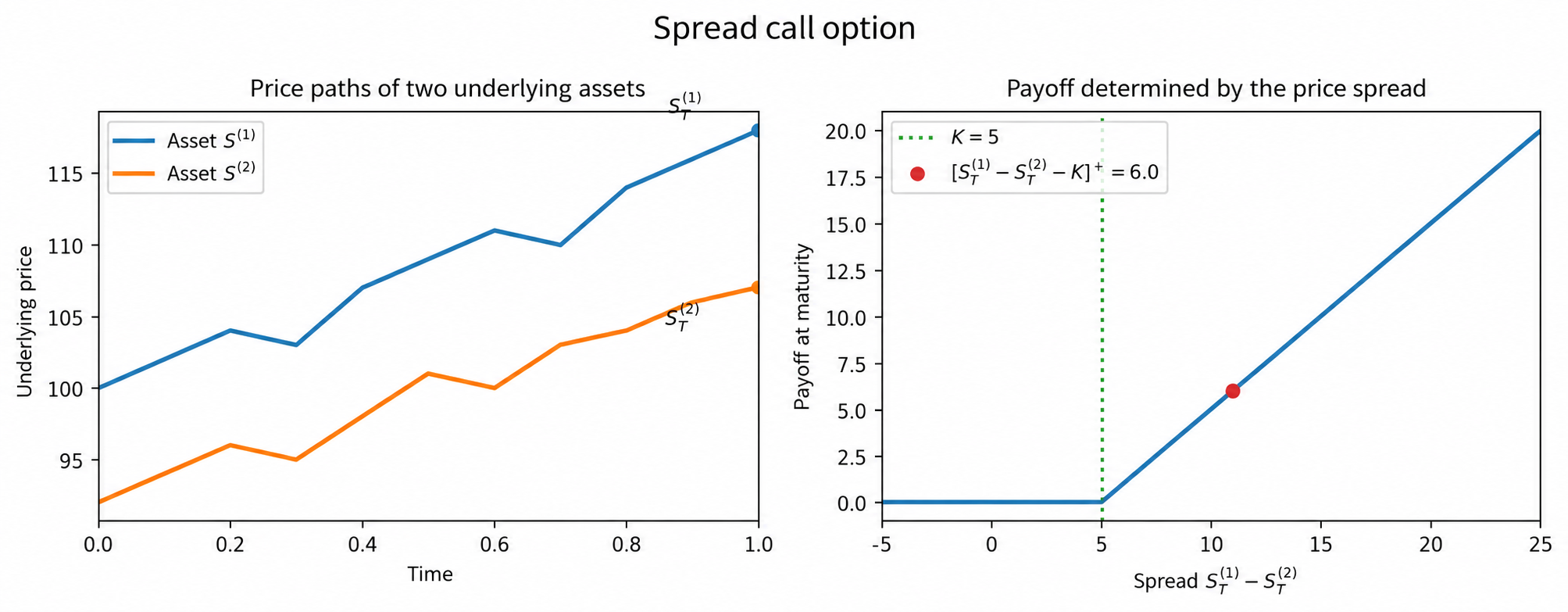
Figure 1.1b Schematic of a spread call option: the payoff is determined by the price difference \(S_T^{(1)}-S_T^{(2)}\) between two underlying assets.
We first develop the pricing theory and methods for European call and put options. Later chapters will address American options, path-dependent options, and options on multiple underlying assets.
1.2 Stochastic Processes for Asset Prices
Let the current time be \(t=0\). We consider options on a stock. The main factor determining the price of a European option is the underlying stock price at maturity \(t=T\), denoted by \(S_T\). The prices of American and Asian options also depend on the history of the underlying asset price up to maturity \(T\), namely \(S_t,0 \leq t\leq T\).
At \(t=0\), future stock prices \(S_t,t>0\) are unknown. For any fixed future time \(t>0\), the asset price \(S_t\) is therefore a random variable. The collection of asset prices \(S_t\) over \((0,T]\) forms a stochastic process. We therefore need to choose a stochastic process to describe stock prices.
At the beginning of the twentieth century, Bachelier (1900) proposed using Brownian motion (see Section 1.3) to describe stock prices. In this model, for any time \(t>0\), the stock price \(S_t\) follows a normal distribution. Since the normal distribution has support \((-\infty,+\infty)\), the model permits negative stock prices.
To ensure positive stock prices, Samuelson (1965) proposed using Brownian motion to describe log returns,
\[X_t=\log S_t-\log S_0\tag{1.2.1}\]
rather than stock prices themselves. The stock price \(\{S_t=S_0\exp(X_t);0<t\leq T\}\) then follows geometric Brownian motion.
Log returns are approximately equal to simple returns (\(X_t'=S_t/S_0-1\)) when price changes are small, as shown by the Taylor expansion of the exponential function, \(e^X \approx 1+X\). The advantages of log returns are as follows:
- The exponential form \(S_t=S_0e^{X_t}\) keeps stock prices positive;
- The total log return over multiple periods equals the sum of the log returns for the individual periods. Consider the following example. Suppose \(S_1=S_0e^{X_1}\), \(S_2=S_1e^{X_2}\), and \(S_3=S_2e^{X_3}\); then \(S_3\) can also be written as \(S_3=S_0e^{X_1+X_2+X_3}\). Moreover, when \(X_1,X_2,X_3\) are independent and normally distributed, \(X_1+X_2+X_3\) is also normally distributed. For simple returns, if \(S_1=S_0(1+X_1')\), \(S_2=S_1(1+X_2')\), and \(S_3=S_2(1+X_3')\), we obtain \(S_3=S_0(1+X_1')(1+X_2')(1+X_3')=S_0(1+X_1'+X_2'+X_3'+X_1'X_2'+X_2'X_3'+X_1'X_3'+X_1'X_2'X_3')\), which contains cross-products absent from the sum of log returns. Furthermore, when \(X_1',X_2',X_3'\) are independent and normally distributed, terms such as \(X_1'X_2'\) are not normally distributed, so the probability distributions of \(S_2,S_3\) are much more complicated than those obtained by adding normal log returns.
We next introduce four stochastic processes for \(X_t\): Brownian motion, jump diffusion, the Variance Gamma process, and the Normal Inverse Gaussian process.
1.3 Brownian Motion
Let \(N(\mu,\sigma^2)\) denote the normal distribution (also called the Gaussian distribution) with mean \(\mu\) and variance \(\sigma^2\). For a random variable \(X\) with distribution \(N(\mu,\sigma^2)\), the probability density function of \(X\) is
\[f(x;\mu,\sigma)=\frac{1}{\sqrt{2\pi}\sigma} \exp\left(-\frac{(x-\mu)^2}{2\sigma^2}\right).\]
When \(\mu=0\) and \(\sigma=1\), \(X\) is said to follow the standard normal distribution, with density denoted by \(\phi(x)\) and distribution function by \(\Phi(x)\). Figure 1.2 shows normal densities with different means and standard deviations. The densities have the following properties:
- The normal density is bell-shaped.
- The distribution is symmetric about its mean \(\mu\). This location parameter determines the center of the distribution; increasing it shifts the curve to the right.
- The standard deviation \(\sigma\) determines the spread of the distribution. Increasing it broadens the distribution and extends its tails.
# Figure 1.2: Normal densities for different means and variances
normal_grid = np.linspace(-6.0, 6.0, 500)
fig, ax = plt.subplots(figsize=(7, 4))
ax.plot(normal_grid, norm.pdf(normal_grid), color="red",
        label=r"$\mu=0,\sigma^2=1$")
ax.plot(normal_grid, norm.pdf(normal_grid, loc=1.0),
        color="blue", linestyle="--", label=r"$\mu=1,\sigma^2=1$")
ax.plot(normal_grid, norm.pdf(normal_grid, scale=np.sqrt(2)),
        color="black", linestyle="-.", label=r"$\mu=0,\sigma^2=2$")
ax.set_xlim(-6, 6)
ax.set_ylim(0, 0.4)
ax.set_xticks(np.arange(-6, 7, 2))
ax.set_yticks(np.arange(0, 0.401, 0.05))
ax.tick_params(direction="in", top=True, right=True)
ax.legend(loc="upper right", frameon=True, fancybox=False,
          facecolor="white", edgecolor="black")
fig.tight_layout()
plt.show()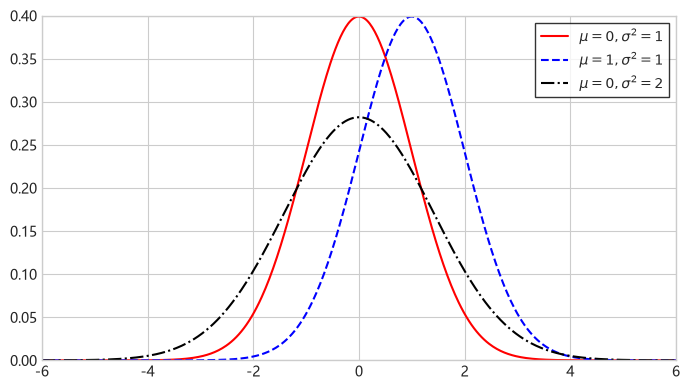
Figure 1.2 Normal probability density functions with different parameters.
Standard Brownian motion (also called a Wiener process) satisfies the following conditions:
- \(W_0=0\);
- The increments of \(W\) are independent: for any times \(t_1<t_2\leq t_3<t_4\), \(W_{t_4}-W_{t_3}\) and \(W_{t_2}-W_{t_1}\) are independent;
- The increments of \(W\) are normally distributed: for all \(t_2>t_1\), \(W_{t_2}-W_{t_1}\sim\mathcal{N}(0,t_2-t_1)\);
- The paths of \(W\) are continuous, with no jumps.
With constants \(\mu\) and \(\sigma\), the process \(X_t=\mu t+\sigma W_t\) is called Brownian motion with drift. For \(X_t\), over an interval of length \(h>0\), the increment \(X_h=X_{t+h}-X_t\) has a normal marginal distribution, \(X_h\sim\mathcal{N}(\mu h,\sigma^2h)\). Thus \(\mu\) is the drift rate, or mean increment per unit time. The volatility \(\sigma\) is the standard deviation of an increment over a unit time interval. The increment mean grows in proportion to \(h\), while its standard deviation grows in proportion to \(\sqrt h\): increasing the interval from 1 year to 4 years multiplies the mean by 4 and the standard deviation by 2.
Figure 1.3 shows five sample paths of \(X_t\) with parameters \(\mu=0.1,\sigma=0.3\).
# Sample paths of Brownian motion with drift
brownian_rng = np.random.default_rng(42)
brownian_steps = 500
brownian_paths_count = 5
brownian_time = np.linspace(0.0, 1.0, brownian_steps + 1)
brownian_dt = brownian_time[1] - brownian_time[0]
brownian_drift = 0.10
brownian_volatility = 0.30
brownian_increments = (
    brownian_drift * brownian_dt
    + brownian_volatility
    * np.sqrt(brownian_dt)
    * brownian_rng.standard_normal(
        (brownian_paths_count, brownian_steps)
    )
)
drifted_brownian_paths = np.column_stack(
    [np.zeros(brownian_paths_count), np.cumsum(brownian_increments, axis=1)]
)
# Figure 1.3: Sample paths of Brownian motion with drift
fig, ax = plt.subplots(figsize=(8, 4.2))
ax.plot(brownian_time, drifted_brownian_paths.T, alpha=0.25)
ax.set_xlabel("Time")
ax.set_ylabel("$X_t$")
ax.set_title("Sample paths of Brownian motion with drift")
ax.grid(True, alpha=0.25)
fig.tight_layout()
plt.show()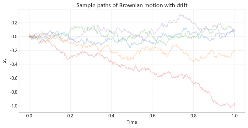
Figure 1.3 Sample paths of Brownian motion with drift.
In Figure 1.4, the blue solid curves show the marginal distributions \(X_t\sim\mathcal{N}(\mu t,\sigma^2t)\) at \(t=1,3,5\). For \(t\in[0,6]\), the black solid line shows the mean and the red dashed lines mark the boundaries of an interval containing approximately 95% of the distribution at each time. This interval is given by \(\mu t\pm1.96\sigma\sqrt t\). As time \(t\) increases, the distribution of \(X_t\) becomes more dispersed.
# Figure 1.4: Marginal distributions of Brownian motion with drift at different times
brownian_marginal_times = np.array([1.0, 3.0, 5.0])
marginal_grid = np.linspace(-1.5, 2.2, 500)
marginal_densities = [
    norm.pdf(
        marginal_grid,
        loc=brownian_drift * time_value,
        scale=brownian_volatility * np.sqrt(time_value),
    )
    for time_value in brownian_marginal_times
]
marginal_mean = brownian_drift * brownian_time
marginal_lower = marginal_mean - 1.96 * brownian_volatility * np.sqrt(
    brownian_time
)
marginal_upper = marginal_mean + 1.96 * brownian_volatility * np.sqrt(
    brownian_time
)
marginal_path_rng = np.random.default_rng(43)
marginal_path_time = np.linspace(0.0, 6.0, 601)
marginal_path_dt = marginal_path_time[1] - marginal_path_time[0]
marginal_path_count = 20
marginal_path_increments = (
    brownian_drift * marginal_path_dt
    + brownian_volatility
    * np.sqrt(marginal_path_dt)
    * marginal_path_rng.standard_normal((marginal_path_count, 600))
)
marginal_paths = np.column_stack(
    [
        np.zeros(marginal_path_count),
        np.cumsum(marginal_path_increments, axis=1),
    ]
)
marginal_path_mean = brownian_drift * marginal_path_time
marginal_path_lower = marginal_path_mean - 1.96 * brownian_volatility * np.sqrt(
    marginal_path_time
)
marginal_path_upper = marginal_path_mean + 1.96 * brownian_volatility * np.sqrt(
    marginal_path_time
)

fig = plt.figure(figsize=(8, 5.5))
ax = fig.add_subplot(111, projection="3d")
for time_value, density in zip(brownian_marginal_times, marginal_densities):
    ax.plot(
        np.full_like(marginal_grid, time_value),
        marginal_grid,
        density,
        color="tab:blue",
    )
ax.plot(
    marginal_path_time,
    marginal_path_mean,
    np.zeros_like(marginal_path_time),
    color="black",
)
ax.plot(
    marginal_path_time,
    marginal_path_lower,
    np.zeros_like(marginal_path_time),
    color="red",
    linestyle="--",
)
ax.plot(
    marginal_path_time,
    marginal_path_upper,
    np.zeros_like(marginal_path_time),
    color="red",
    linestyle="--",
)
for path in marginal_paths:
    ax.plot(
        marginal_path_time,
        path,
        np.zeros_like(marginal_path_time),
        color="limegreen",
        linestyle="--",
        alpha=0.35,
    )
ax.set_xlabel("$t$")
ax.set_ylabel("$X_t$")
ax.set_zlabel("pdf")
ax.set_title("Marginal distributions of Brownian motion with drift")
fig.tight_layout()
plt.show()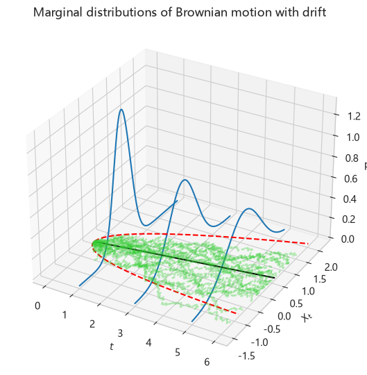
Figure 1.4 Marginal distributions of Brownian motion with drift at different times.
Let \(\mu_1\) denote the mean and \(\mu_k\) (for \(k=2,3,4\)) the second through fourth central moments. The moments of a normal random variable are given by: \[ \begin{aligned} \mu_1 &= E [X_h] = \mu h,\\ \mu_2 &= E [(X_h - E[X_h])^2] = \sigma^2 h,\\ \mu_3 &= E [(X_h - E[X_h])^3] = 0,\\ \mu_4 &= E [(X_h - E[X_h])^4] = 3\sigma^4 h^2. \end{aligned} \]
The first moment is the mean, and the second central moment is the variance. Standardizing the third and fourth moments gives two further characteristics of the distribution: skewness and kurtosis. They are defined as follows:
\[ \begin{aligned} Skw &:= \frac{\mu_3}{\mu_2^{3/2}}, \quad Krt := \frac{\mu_4}{\mu_2^2}. \end{aligned} \]
The normal distribution has skewness 0 and kurtosis 3. Subtracting 3 from kurtosis gives excess kurtosis, which is 0 for the normal distribution. When the relevant moments exist, a symmetric distribution has skewness 0. A distribution with kurtosis greater than 3 (excess kurtosis greater than 0) is called leptokurtic. Kurtosis is the average of the fourth powers of standardized deviations, which makes it particularly sensitive to extreme values: an observation 4 standard deviations from the mean contributes \(4^4=256\), while one 2 standard deviations away contributes \(2^4=16\), a factor of 16 smaller.
When \(X_t=\mu t+\sigma W_t\) describes stock log returns, the stock price
\[\frac{S_t}{S_0}=e^{X_t}=e^{\mu t+\sigma W_t}\]
follows geometric Brownian motion. At any given time \(t\), the marginal distribution of \(S_t/S_0\) is lognormal:
\[\frac{S_t}{S_0}\sim\operatorname{Lognormal}(\mu t,\sigma^2t).\]
Using the moments of the lognormal distribution, we obtain the following expressions for the expectation and variance of \(S_t/S_0\), respectively:
\[E\left[\frac{S_t}{S_0}\right]=\frac{E[S_t]}{S_0}=e^{(\mu+\sigma^2/2)t},\]
\[\begin{aligned} \operatorname{Var}\left[\frac{S_t}{S_0}\right] &=E\left[\left(\frac{S_t}{S_0}\right)^2\right]-E\left[\frac{S_t}{S_0}\right]^2 \\ &=e^{2(\mu+\sigma^2)t}-e^{(2\mu+\sigma^2)t} \\ &=e^{(2\mu+\sigma^2)t}(e^{\sigma^2t}-1). \end{aligned}\]
This model was first proposed by Samuelson (1965), so it is also called the Samuelson model.
Note that \(\mu\) is the drift rate of the log return \(X_t\), with \(E[X_t]=\mu t\). The expected stock price grows at rate \(\mu+\sigma^2/2\) instead of \(\mu\), because the normal random component satisfies \(E[e^{\sigma W_t}]=e^{\sigma^2t/2}\), giving \(E[S_t]/S_0=e^{(\mu+\sigma^2/2)t}\).
1.3.1 Fitting Geometric Brownian Motion to the S&P 500 Index
We next fit geometric Brownian motion to the S&P 500 index from January 1, 2000, to June 28, 2013, using the method of moments.
Historical S&P 500 index data can be obtained from Yahoo Finance. The following code downloads the ^GSPC series from January 2000 through June 28, 2013. The downloaded data remain in memory during the current session for use in later calculations in this chapter. Yahoo Finance excludes the end date from the download interval, so the code sets end to 2013-06-29. With auto_adjust=False, the code selects the Adj Close field and renames it close to provide a consistent price variable for subsequent formulas. For individual stocks, Adjusted Close includes adjustments for splits and dividends.
# Download historical S&P 500 data
sp500_data = yf.download(
    "^GSPC", start="2000-01-01", end="2013-06-29",
    auto_adjust=False, multi_level_index=False, progress=False,
)
sp500_data = sp500_data.rename_axis("date").reset_index()
sp500_data["close"] = pd.to_numeric(sp500_data["Adj Close"])
sp500_data = (
    sp500_data[["date", "close"]]
    .sort_values("date")
    .dropna(subset=["close"])
    .reset_index(drop=True)
)
print("Data source: Yahoo Finance: ^GSPC Adj Close (current download)")
print(f"Observations: {len(sp500_data):,}; interval: "
      f"{sp500_data['date'].iloc[0]:%Y-%m-%d} to "
      f"{sp500_data['date'].iloc[-1]:%Y-%m-%d}")
sp500_data.head()
Data source: Yahoo Finance: ^GSPC Adj Close (current download)
Observations: 3,393; interval: 2000-01-03 to 2013-06-28| date | close | |
|---|---|---|
| 0 | 2000-01-03 | 1455.219971 |
| 1 | 2000-01-04 | 1399.420044 |
| 2 | 2000-01-05 | 1402.109985 |
| 3 | 2000-01-06 | 1403.449951 |
| 4 | 2000-01-07 | 1441.469971 |
# Figure 1.5: S&P 500 adjusted closing prices from January 2000 to June 2013
fig, ax = plt.subplots(figsize=(10, 4.2))
ax.plot(sp500_data["date"], sp500_data["close"])
ax.set_xlabel("Date")
ax.set_ylabel("Index level")
ax.set_title("S&P 500 adjusted close")
plt.show()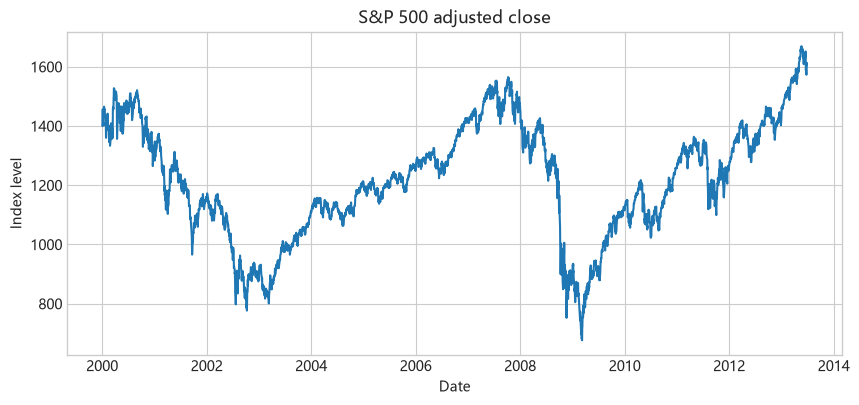
Figure 1.5 Adjusted closing price series of the S&P 500 from January 2000 to June 2013.
Common stock index tickers on Yahoo Finance are listed below. To download another index, simply replace the ticker in yf.download with the corresponding value in the table.
| Yahoo Finance ticker | Stock index |
|---|---|
^GSPC |
S&P 500 |
^DJI |
Dow Jones Industrial Average |
^IXIC |
Nasdaq Composite |
^FTSE |
FTSE 100 |
^GDAXI |
DAX |
^FCHI |
CAC 40 |
^STOXX50E |
Euro Stoxx 50 |
^HSI |
Hang Seng Index |
000001.SS |
Shanghai Composite |
^N225 |
Nikkei 225 |
Table 1.1 Common stock index tickers on Yahoo Finance.
We analyse the daily adjusted closing prices by first calculating the daily log returns. Figure 1.6 shows S&P 500 index log returns from January 2000 to June 2013.
\[ x_i=\log(S_i)-\log(S_{i-1}),\quad i=1,\ldots,n \tag{1.3.1} \]
# Calculate daily log returns
log_returns = np.diff(np.log(sp500_data["close"].to_numpy()))
return_dates = sp500_data["date"].iloc[1:]
# Figure 1.6: Daily S&P 500 log returns from January 2000 to June 2013
fig, ax = plt.subplots(figsize=(10, 4.2))
ax.plot(return_dates, log_returns)
ax.set_xlabel("Date")
ax.set_ylabel("Log return")
ax.set_title("S&P 500 daily log returns")
plt.show()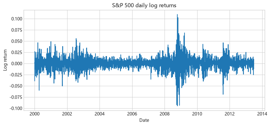
Figure 1.6 Daily log returns of the S&P 500 from January 2000 to June 2013.
Throughout this chapter, we estimate parameters from empirical central moments: the second- and higher-order central moments are calculated using \(n\) as the denominator, and skewness and kurtosis are calculated directly from these central moments, without additional finite-sample bias correction. We first calculate the sample mean and variance of log returns,
\[ \widehat\mu_{1,n}=\frac{1}{n}\sum_{i=1}^n x_i,\quad \widehat{\operatorname{Var}}_n=\frac{1}{n} \sum_{i=1}^n(x_i-\widehat\mu_{1,n})^2.\]
We then calculate the sampling interval \(h=T/n\), where \(T\) is the duration of the sample period. GBM assumes that daily log returns follow \(\mathcal{N}(\mu h,\sigma^2h)\), so the sample mean and sample variance give
\[ \widehat\mu=\frac{\widehat\mu_{1,n}}{h},\quad \widehat\sigma=\sqrt{\frac{\widehat{\operatorname{Var}}_n}{h}}.\]
Here \(h\) is the length of the observation period in calendar time divided by the number of return increments, so it is the average observation interval in years, approximately \(1/252\). To express the parameters on a yearly basis, we divide the mean daily log return by \(h\) and its standard deviation by \(\sqrt h\), because variance is proportional to the time interval. For example, with \(h=1/252\), a daily return standard deviation of \(1\%\) corresponds to annualized volatility of approximately \(1\%\times\sqrt{252}=15.9\%\). The following code implements these steps.
# Calculate GBM moment estimates and sample statistics
sample_years = (
    sp500_data["date"].iloc[-1] - sp500_data["date"].iloc[0]
).days / 365.25
time_step = sample_years / len(log_returns)
sample_mean = np.mean(log_returns)
sample_variance = np.var(log_returns, ddof=0)
drift = sample_mean / time_step
volatility = np.sqrt(sample_variance / time_step)
sample_skewness = skew(log_returns, bias=True)
sample_kurtosis = kurtosis(log_returns, fisher=False, bias=True)
sample_excess_kurtosis = sample_kurtosis - 3.0
pd.Series(
    {
        "Time step": time_step,
        "Drift rate": drift,
        "Volatility": volatility,
        "Skewness": sample_skewness,
        "Kurtosis": sample_kurtosis,
    }
)
Time step 0.003975
Drift rate 0.007325
Volatility 0.211596
Skewness -0.167776
Kurtosis 10.469578
dtype: float64The drift rate and volatility obtained by the method of moments are shown in the program output above. The sample kurtosis is approximately 10.5, far above the normal distribution’s kurtosis of 3, indicating heavy tails in S&P 500 index log returns. Figure 1.7 shows the normal fit to daily log returns. The S&P 500 log-return distribution has a sharp peak and heavy tails, and the normal distribution substantially underestimates the probability of extreme returns.
Thus, the normal distribution does not adequately describe daily S&P 500 index log returns. Sections 1.4 to 1.6 therefore introduce three stochastic processes that provide better fits: the Merton jump diffusion model, the Variance Gamma model, and the Normal Inverse Gaussian model. The main difference between these models and geometric Brownian motion is that all three include jumps, whereas geometric Brownian motion has continuous paths.
# Figure 1.7: Normal fit to the overall distribution and left tail of daily S&P 500 log returns
normal_lower = -0.10
normal_upper = 0.11
normal_bin_count = 50
normal_bin_width = (normal_upper - normal_lower) / normal_bin_count
fit_bin_edges = np.linspace(normal_lower, normal_upper, normal_bin_count + 1)
fit_bin_centres = (fit_bin_edges[:-1] + fit_bin_edges[1:]) / 2
normal_grid = fit_bin_centres
normal_bin_counts = len(log_returns) * np.diff(
    norm.cdf(fit_bin_edges, loc=sample_mean, scale=np.sqrt(sample_variance))
)
fitted_normal = normal_bin_counts

def model_bin_counts(density, centre=None):
    """Integrate each density over the common bins, splitting at a singularity."""
    return len(log_returns) * np.array([
        quad(density, left, right,
             points=[centre] if centre is not None and left < centre < right else None)[0]
        for left, right in zip(fit_bin_edges[:-1], fit_bin_edges[1:])
    ])

left_tail_cutoff = -0.02
left_tail_lower = -0.10
left_tail_bin_count = normal_bin_count
left_tail_grid = np.linspace(left_tail_lower, left_tail_cutoff, 300)
left_tail_normal = (
    norm.pdf(
        left_tail_grid,
        loc=sample_mean,
        scale=np.sqrt(sample_variance),
    )
    * len(log_returns)
    * normal_bin_width
)
fig, axes = plt.subplots(1, 2, figsize=(11, 4.2))
axes[0].hist(
    log_returns,
    bins=fit_bin_edges,
    range=(normal_lower, normal_upper),
    color="0.75",
    edgecolor="blue",
    linewidth=0.8,
    label="Sample returns",
)
axes[0].plot(
    normal_grid,
    fitted_normal,
    color="red",
    linewidth=1.8,
    label="GBM expected counts",
)
axes[0].set_xlabel("Log return")
axes[0].set_ylabel("Count")
axes[0].set_title("Overall distribution")
axes[0].set_xlim(normal_lower, normal_upper)
axes[0].grid(True, alpha=0.25)
axes[0].legend(frameon=False)

axes[1].hist(
    log_returns,
    bins=fit_bin_edges,
    range=(normal_lower, normal_upper),
    color="0.75",
    edgecolor="blue",
    linewidth=0.8,
    label="Sample returns",
)
axes[1].plot(
    left_tail_grid,
    left_tail_normal,
    color="red",
    linewidth=1.8,
    label="GBM expected counts",
)
axes[1].set_xlabel("Log return")
axes[1].set_ylabel("Count")
axes[1].set_title("Left tail")
axes[1].set_xlim(left_tail_lower, left_tail_cutoff)
axes[1].set_xticks(np.arange(-0.10, -0.019, 0.02))
axes[1].set_ylim(0.0, 50.0)
axes[1].grid(True, alpha=0.25)
axes[1].legend(frameon=False)
fig.tight_layout()
plt.show()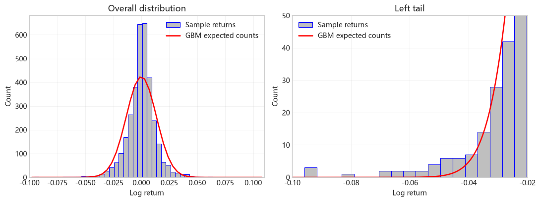
Figure 1.7 GBM fit to S&P 500 index log returns from January 2000 to June 2013.
1.4 Merton Jump Diffusion Model
To improve the fit to historical daily S&P 500 log returns, we can add random jumps to Brownian motion with drift:
\[X_t=\mu t+\sigma W_t+\sum_{i=1}^{N_t}J_i.\]
Here, \(\sum_{i=1}^{N_t}J_i\) represents a compound Poisson process. A compound Poisson process has two sources of randomness. First, the Poisson process determines the random jump times. \(N_t\) represents the number of jumps in \([0,t]\) and follows a Poisson distribution with mean \(\lambda t\):
\[P(N_t=n)=\frac{e^{-\lambda t}(\lambda t)^n}{n!},\quad n=0,1,\ldots.\]
The jump intensity \(\lambda\) measures the rate at which jumps occur. When time is measured in years, \(\lambda\) is quoted per year. Over an interval of length \(h\), the expected number of jumps is \(E[N_h]=\lambda h\), and the probability of at least one jump is \(1-e^{-\lambda h}\). For a short interval with \(\lambda h\ll1\), this probability is approximately \(\lambda h\). For example, when \(\lambda=12\) and \(h=1/12\), there is on average one jump per month, but the probability of no jumps is still \(e^{-1}\approx36.8\%\).
Second, the jump sizes \(J_i\) (\(i=1,\ldots,N_t\)) are independent and identically distributed random variables. The Poisson process, jump sizes, and Brownian motion are all assumed to be mutually independent. Merton (1976) proposed normally distributed jump sizes \(J_i\), while Kou (2002) used a double exponential distribution to describe jump sizes, with the sizes of positive and negative jumps each following an exponential distribution conditional on their sign.
In this section we use the jump diffusion model proposed by Merton (1976), in which jump sizes follow the normal distribution \(J_i\sim\mathcal{N}(a,b^2)\). The parameter \(a\) is the mean log jump size, and \(b\) is its standard deviation. A single log jump \(J\) multiplies the stock price by \(e^J\). Holding other parameters fixed, increasing \(\lambda\) increases the frequency of jumps, while increasing \(b\) increases the dispersion of individual jump sizes. Figure 1.8 shows five sample paths of the log-return process \(X_t\) in the Merton jump diffusion model.
# Figure 1.8: Set parameters for five Merton log-return paths
merton_path_rng = np.random.default_rng(17)
merton_path_count = 5
merton_path_step_count = 252
merton_path_time = np.linspace(
    0.0, 1.0, merton_path_step_count + 1
)
merton_path_dt = merton_path_time[1] - merton_path_time[0]
merton_path_drift = 0.08
merton_path_volatility = 0.20
merton_path_jump_intensity = 12.0
merton_path_jump_mean = 0.0
merton_path_jump_std = 0.06
# Figure 1.8: Generate Brownian increments and Poisson jumps, then accumulate the paths
merton_path_normals = merton_path_rng.standard_normal(
(merton_path_count, merton_path_step_count)
)
merton_path_jump_counts = merton_path_rng.poisson(
merton_path_jump_intensity * merton_path_dt,
size=(merton_path_count, merton_path_step_count),
)
merton_path_jump_sizes = (
merton_path_jump_counts * merton_path_jump_mean
+ merton_path_jump_std
* np.sqrt(merton_path_jump_counts)
* merton_path_rng.standard_normal(
(merton_path_count, merton_path_step_count)
)
)
merton_path_increments = (
merton_path_drift * merton_path_dt
+ merton_path_volatility * np.sqrt(merton_path_dt) * merton_path_normals
+ merton_path_jump_sizes
)
merton_log_paths = np.column_stack(
[np.zeros(merton_path_count), np.cumsum(merton_path_increments, axis=1)]
)# Figure 1.8: Sample paths of the Merton jump diffusion log-return process
fig, ax = plt.subplots(figsize=(8, 4.2))
jump_label_added = False
for path_index, path in enumerate(merton_log_paths):
(line,) = ax.plot(
merton_path_time,
path,
alpha=0.80,
)
jump_steps = np.flatnonzero(merton_path_jump_counts[path_index] > 0) + 1
if len(jump_steps) > 0:
ax.scatter(
merton_path_time[jump_steps],
path[jump_steps],
color=line.get_color(),
s=18,
zorder=3,
label="Jump times" if not jump_label_added else None,
)
jump_label_added = True
ax.set_xlabel("Time")
ax.set_ylabel("Log-return process $X_t$")
ax.set_title("Log-return paths of Merton jump diffusion")
ax.grid(True, alpha=0.25)
ax.legend(frameon=False)
plt.show()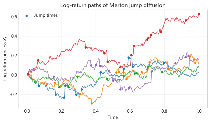
Figure 1.8 Five sample paths of the log-return process \(X_t\) in the Merton jump diffusion model.
Let \(X_h=X_{t+h}-X_t\) denote the increment over an interval of length \(h>0\), and let \(N_h=N_{t+h}-N_t\) count the jumps during \((t,t+h]\). If exactly \(n\) jumps occur, we can write the increment as
\[ X_h=\underbrace{\mu h}_{\text{drift}}+\underbrace{\sigma(W_{t+h}-W_t)}_{\text{diffusion}}+\underbrace{\sum_{i=1}^{N_h}J_i}_{\text{total jump contribution}}. \]
Here \(J_i=a+bZ_i\) is the size of jump \(i\), with independent standard normal variables \(Z_i\sim\mathcal{N}(0,1)\). The parameter \(a\) is the mean jump size, and \(b\geq0\) is its standard deviation. When \(n=0\), the jump contribution is zero.
The Brownian increment satisfies \(W_{t+h}-W_t\sim\mathcal{N}(0,h)\) and is independent of the jump count and jump sizes. Given \(n\) jumps, the jump sum has mean \(na\) and variance \(nb^2\). Adding the independent diffusion component gives the conditional distribution
\[ X_h\mid N_h=n\sim\mathcal{N}(\mu h+an,\;\sigma^2h+nb^2). \]
Weighting the conditional normal densities by the jump-count probabilities gives the unconditional probability density function of \(X_h\):
\[ \begin{aligned} f_{X_h}(x) &=\sum_{n=0}^{\infty} \frac{e^{-\lambda h}(\lambda h)^n}{n!} \frac{1}{\sqrt{2\pi(\sigma^2h+nb^2)}}\\ &\quad\times\exp\left(-\frac{\left[x-(\mu h+na)\right]^2} {2(\sigma^2h+nb^2)}\right). \end{aligned} \]
The density is an infinite mixture of normal distributions (see Aït-Sahalia (2004)). We approximate this density by truncating the sum at a sufficiently large jump count \(N_{\max}\). Let \(\varepsilon\) be the maximum probability mass to omit from the right tail of the Poisson distribution, and let \(F^{-1}_{\operatorname{Pois}(\lambda h)}\) denote the quantile function of the Poisson distribution with mean \(\lambda h\). Take
\[ N_{\max}=F^{-1}_{\operatorname{Pois}(\lambda h)}(1-\varepsilon), \qquad f_{X_h}(x)\approx\sum_{n=0}^{N_{\max}}P(N_h=n)\,f_{X_h\mid N_h=n}(x). \]
That is, the calculation retains the normal mixture terms for \(n=0,1,\ldots,N_{\max}\) and discards those for \(n>N_{\max}\); the discarded weight satisfies \(P(N_h>N_{\max})\leq\varepsilon\). See Function 1.1 for the implementation, with \(\varepsilon=10^{-12}\) by default.
From Formulas to Code
drift, diffusion_volatility, jump_intensity, jump_mean, and jump_std correspond to \(\mu,\sigma,\lambda,a,b\), respectively; time_horizon corresponds to the increment length \(h\).
jump_count corresponds to the jump count \(n\); conditional_mean and conditional_std are \(\mu h+na\) and \(\sqrt{\sigma^2h+nb^2}\), respectively. The program sums the conditional normal densities weighted by Poisson probabilities.
Function 1.1: Merton increment density
def merton_increment_density(
    x, drift, diffusion_volatility, jump_intensity,
    jump_mean, jump_std, time_horizon, tail_probability=1e-12,
):
    '''Evaluate the Merton increment density by a truncated Poisson mixture.

    The infinite mixture is truncated after a Poisson quantile. The
    omitted probability mass is at most tail_probability.
    '''
    expected_jump_count = jump_intensity * time_horizon
    maximum_jump_count = int(
        poisson.ppf(1.0 - tail_probability, expected_jump_count)
    )
    density = 0.0
    for jump_count in range(maximum_jump_count + 1):
        conditional_mean = drift * time_horizon + jump_count * jump_mean
        conditional_std = np.sqrt(
            diffusion_volatility**2 * time_horizon
            + jump_count * jump_std**2
        )
        density += poisson.pmf(jump_count, expected_jump_count) * norm.pdf(
            x, loc=conditional_mean, scale=conditional_std
        )
    return density
The mean and second- through fourth-order central moments of \(X_h\) are, respectively,
\[ \begin{aligned} \mu_1 &= E[X_h] = (\mu+\lambda a)h,\\ \mu_2 &= E[(X_h-E[X_h])^2] = (\sigma^2+\lambda a^2+\lambda b^2)h,\\ \mu_3 &= E[(X_h-E[X_h])^3] = \lambda a(a^2+3b^2)h,\\ \mu_4 &= E[(X_h-E[X_h])^4] = \lambda(a^4+6a^2b^2+3b^4)h+3\mu_2^2. \end{aligned} \]
1.4.1 Moment Estimation for the Merton Jump Diffusion Model
Beckers (1981) derived moment estimators for the Merton jump diffusion model using cumulants. If two random variables have identical moments of every order, their cumulants are also identical, and vice versa. Thus, the cumulants of a random variable provide the same information as its moments. For normal Brownian increments, cumulants of order greater than two are zero; after adding jumps, higher-order cumulants reflect information about the jump component. Therefore, the estimation below uses cumulants of orders two through six to distinguish continuous volatility from jump frequency and jump size.
Cumulants are defined through the cumulant-generating function, which will be introduced in Section 5.1.1. Here we use the relationships between the first six cumulants and the central moments. Let \(\kappa_n\) denote the \(n\)th cumulant. When the first six moments exist, the following equations hold:
\[ \begin{aligned} \kappa_1 &= \mu_1,\\ \kappa_2 &= \mu_2,\\ \kappa_3 &= \mu_3,\\ \kappa_4 &= \mu_4-3\mu_2^2,\\ \kappa_5 &= \mu_5-10\mu_3\mu_2,\\ \kappa_6 &= \mu_6-15\mu_4\mu_2-10\mu_3^2+30\mu_2^3. \end{aligned} \]
Assuming \(a=0\) in the Merton jump diffusion model, the equations above simplify to
\[ \begin{aligned} \kappa_1 &= \mu h,\\ \kappa_2 &= (\sigma^2+\lambda b^2)h,\\ \kappa_3 &= \kappa_5=0,\\ \kappa_4 &= 3b^4\lambda h,\\ \kappa_6 &= 15b^6\lambda h. \end{aligned} \]
Solving these equations gives the following moment estimators for the parameters:
\[ \widehat\mu=\frac{\widehat\kappa_1}{h},\quad \widehat\lambda=\frac{25\widehat\kappa_4^3}{3\widehat\kappa_6^2h},\quad \widehat b^2=\frac{\widehat\kappa_6}{5\widehat\kappa_4},\quad \widehat\sigma^2=\frac{\widehat\kappa_2}{h}-\frac{5\widehat\kappa_4^2}{3\widehat\kappa_6h}. \]
Function 1.2 implements these estimators. It calculates even-order moments under the symmetric model \(a=0\) and sets odd-order central moments to zero. Its sixth-order cumulant therefore omits the \(-10\mu_3^2\) term in the general formula; this constraint is imposed to simplify estimation.
From Formulas to Code
time_step corresponds to the time interval \(h\) between adjacent observations; cumulant_1, cumulant_2, cumulant_4, and cumulant_6 store the first-, second-, fourth-, and sixth-order cumulants calculated from the sample.
Under the specification \(a=0\), the returned drift, jump_intensity, jump_std, and diffusion_volatility correspond to \(\hat\mu,\hat\lambda,\hat b,\hat\sigma\), respectively.
Function 1.2: Merton parameter estimation from cumulants
def fit_merton_moments(log_returns, time_step):
    '''Estimate the Merton drift, jump intensity, jump scale, and volatility.

    The estimation uses the simplified Merton specification a=0.
    '''
    sample_mean = np.mean(log_returns)
    sample_variance = np.var(log_returns, ddof=0)
    central_moment_4 = np.mean((log_returns - sample_mean) ** 4)
    central_moment_6 = np.mean((log_returns - sample_mean) ** 6)

    cumulant_1 = sample_mean
    cumulant_2 = sample_variance
    cumulant_4 = central_moment_4 - 3 * sample_variance**2
    cumulant_6 = (
        central_moment_6
        - 15 * central_moment_4 * sample_variance
        + 30 * sample_variance**3
    )

    drift = cumulant_1 / time_step
    jump_intensity = 25 * cumulant_4**3 / (
        3 * cumulant_6**2 * time_step
    )
    jump_std = np.sqrt(cumulant_6 / (5 * cumulant_4))
    diffusion_volatility = np.sqrt(
        (cumulant_2 - 5 * cumulant_4**2 / (3 * cumulant_6))
        / time_step
    )
    return drift, jump_intensity, jump_std, diffusion_volatility
# Use Function 1.2 to estimate Merton model parameters
(
merton_drift,
merton_jump_intensity,
merton_jump_std,
merton_diffusion_volatility,
) = fit_merton_moments(log_returns, time_step)
merton_parameters = pd.Series(
{
"mu (drift rate)": merton_drift,
"lambda (jump intensity)": merton_jump_intensity,
"b (jump standard deviation)": merton_jump_std,
"sigma (diffusion volatility)": merton_diffusion_volatility,
},
name="Merton cumulant-based moment estimates",
)
merton_parametersmu (drift rate) 0.007325
lambda (jump intensity) 18.602054
b (jump standard deviation) 0.032137
sigma (diffusion volatility) 0.159879
Name: Merton cumulant-based moment estimates, dtype: float64# Figure 1.9: Integrate over the common bins to calculate model expected counts
merton_plot_lower, merton_plot_upper = fit_bin_edges[[0, -1]]
merton_bin_count = len(fit_bin_centres)
merton_bin_width = fit_bin_edges[1] - fit_bin_edges[0]
merton_grid = fit_bin_centres
merton_bin_counts = model_bin_counts(
lambda x: merton_increment_density(
x, merton_drift, merton_diffusion_volatility,
merton_jump_intensity, 0.0, merton_jump_std, time_step
)
)
merton_density_counts = merton_bin_counts
fitted_normal = normal_bin_countsThe moment estimates for the Merton model are
\[ \widehat\mu=0.007325,\quad \widehat\sigma=0.159879,\quad \widehat\lambda=18.602054,\quad \widehat b=0.032137. \]
These parameters imply an average of approximately 19 jumps per year. The standard deviation of a single log jump is \(\widehat b=0.032137\), approximately the standard deviation of the Brownian component over 10 trading days.
# Figure 1.9: Merton fit to daily S&P 500 log returns; Merton expected counts in solid red and GBM in dashed blue
fig, ax = plt.subplots(figsize=(8, 4.2))
ax.hist(
    log_returns,
    bins=fit_bin_edges,
    range=(merton_plot_lower, merton_plot_upper),
    color="0.75",
    edgecolor="blue",
    linewidth=0.8,
    label="Sample returns",
)
ax.plot(
    merton_grid,
    merton_density_counts,
    color="red",
    linewidth=1.8,
    label="Merton expected counts",
)
ax.plot(
    merton_grid,
    fitted_normal,
    color="blue",
    linewidth=1.8,
    linestyle="--",
    label="GBM expected counts",
)
ax.set_xlim(merton_plot_lower, merton_plot_upper)
ax.set_xticks(np.arange(-0.10, 0.101, 0.05))
ax.set_xlabel("Log return")
ax.set_ylabel("Count")
ax.set_title("Merton and GBM expected counts")
ax.legend()
plt.show()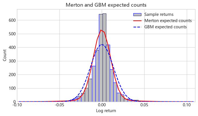
Figure 1.9 Merton jump diffusion model fit to the overall distribution of daily S&P 500 log returns. The red solid line gives the expected count per bin under the Merton model, and the blue dashed line gives the expected count per bin under GBM.
The Merton jump diffusion model substantially improves the fit to the tails of the return distribution compared with the normal distribution, but the peak at the center of the distribution is still not sharp enough.
Figures 1.9a and 1.9b below compare the fits of the Merton jump diffusion model and GBM in the left and right tails.
# Figures 1.9a and 1.9b: Prepare histogram counts for the left and right tail comparisons
tail_bin_edges = fit_bin_edges
tail_bin_centres = (tail_bin_edges[:-1] + tail_bin_edges[1:]) / 2
tail_bin_width = tail_bin_edges[1] - tail_bin_edges[0]
tail_return_grid = np.linspace(
    tail_bin_edges[0], tail_bin_edges[-1], 2000
)
histogram_counts, _ = np.histogram(log_returns, bins=tail_bin_edges)
gbm_expected_counts = (
    norm.pdf(
        tail_return_grid,
        loc=drift * time_step,
        scale=volatility * np.sqrt(time_step),
    )
    * len(log_returns)
    * tail_bin_width
)
Plotting helper function: Comparison of model and GBM densities in the left and right tails
def plot_tail_comparison(
    tail_return_grid,
    tail_bin_centres,
    histogram_counts,
    tail_bin_width,
    gbm_expected_counts,
    model_expected_counts,
    model_label,
    x_limits,
    title,
):
    '''Compare observed tail-bin counts with a model and the GBM benchmark.'''
    grid_in_tail = (
        (tail_return_grid >= x_limits[0])
        & (tail_return_grid <= x_limits[1])
    )
    bins_in_tail = (
        (tail_bin_centres >= x_limits[0])
        & (tail_bin_centres <= x_limits[1])
    )
    fig, ax = plt.subplots(figsize=(8, 4.2))
    ax.bar(
        tail_bin_centres[bins_in_tail],
        histogram_counts[bins_in_tail],
        width=tail_bin_width,
        color="0.75",
        edgecolor="blue",
        linewidth=0.8,
        label="Sample returns",
    )
    ax.plot(
        tail_return_grid[grid_in_tail],
        model_expected_counts[grid_in_tail],
        color="red",
        linewidth=1.8,
        label=model_label,
    )
    ax.plot(
        tail_return_grid[grid_in_tail],
        gbm_expected_counts[grid_in_tail],
        color="blue",
        linewidth=1.8,
        linestyle="--",
        label="GBM normal density",
    )
    ax.set_xlim(*x_limits)
    ax.set_ylim(0.0, 50.0)
    if x_limits[1] <= 0.0:
        ax.set_xticks(np.arange(-0.10, -0.019, 0.02))
    else:
        ax.set_xticks(np.arange(0.02, 0.101, 0.02))
    ax.set_xlabel("Daily log return")
    ax.set_ylabel("Count per bin")
    ax.set_title(title)
    ax.legend(frameon=False)
    fig.tight_layout()
    return fig
# Figure 1.9a: Compare Merton jump diffusion and GBM in the left tail
merton_expected_counts = (
merton_increment_density(
tail_return_grid,
merton_drift,
merton_diffusion_volatility,
merton_jump_intensity,
0.0,
merton_jump_std,
time_step,
)
* len(log_returns)
* tail_bin_width
)
plot_tail_comparison(
tail_return_grid,
tail_bin_centres,
histogram_counts,
tail_bin_width,
gbm_expected_counts,
merton_expected_counts,
"Merton jump diffusion",
(-0.10, -0.02),
"Merton jump diffusion vs. GBM: left tail",
)
plt.show()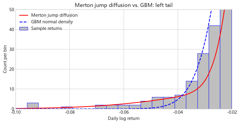
Figure 1.9a Comparison of the Merton jump diffusion model and GBM in the left tail.
# Figure 1.9b: Compare Merton jump diffusion and GBM in the right tail
plot_tail_comparison(
    tail_return_grid,
    tail_bin_centres,
    histogram_counts,
    tail_bin_width,
    gbm_expected_counts,
    merton_expected_counts,
    "Merton jump diffusion",
    (0.02, 0.11),
    "Merton jump diffusion vs. GBM: right tail",
)
plt.show()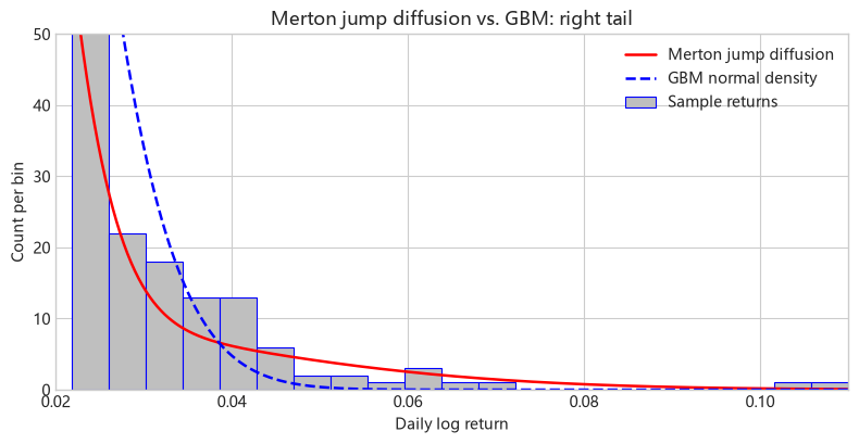
Figure 1.9b Comparison of the Merton jump diffusion model and GBM in the right tail.
1.5 Variance Gamma Model
The Variance Gamma model was proposed by Madan et al. (1998). In this section we fit historical stock returns using the VG process.
1.5.1 Gamma Distribution and Gamma Process
Let \(\gamma(t;\mu,\nu)\) denote a \(Gamma\) process. Over \((t,t+h)\), its increment \(g=\gamma(t+h;\mu,\nu)-\gamma(t;\mu,\nu)\) has mean \(\mu h\) and variance \(\nu h\), and follows a \(Gamma\) distribution with density
\[ f_h(g)=\left(\frac{\mu}{\nu}\right)^{\frac{\mu^2h}{\nu}} \frac{g^{\frac{\mu^2h}{\nu}-1}e^{-\frac{\mu}{\nu}g}} {\Gamma\left(\frac{\mu^2h}{\nu}\right)},\quad g>0. \]
Here, \(\Gamma(\cdot)\) denotes the gamma function \(\Gamma(z)=\int_0^\infty u^{z-1}e^{-u}\,du\).
# Import the numerical, statistical, and plotting libraries used in this section
from scipy.stats import gamma as gamma_distribution
from scipy.special import gammaln, kve

gamma_mean = 1.0
gamma_variance_rate = 0.01
gamma_intervals = [1 / 50, 1 / 250]
gamma_grid = np.linspace(1e-6, 0.10, 500)
From Formulas to Code
increment corresponds to \(g\), and mean_rate, variance_rate, and interval correspond to \(\mu,\nu,h\), respectively. SciPy uses shape and scale parameters: shape corresponds to \(\mu^2h/\nu\), and scale corresponds to \(\nu/\mu\).
Function 1.3: Gamma increment density
def gamma_increment_density(increment, mean_rate, variance_rate, interval):
    '''Evaluate a Gamma increment density from its mean and variance rates.'''
    shape = mean_rate**2 * interval / variance_rate
    scale = variance_rate / mean_rate
    return gamma_distribution.pdf(increment, a=shape, scale=scale)
# Figure 1.10, left: Calculate Gamma increment densities for two time intervals
gamma_densities = [
gamma_increment_density(
gamma_grid, gamma_mean, gamma_variance_rate, interval
)
for interval in gamma_intervals
]# Figure 1.10, right: Set the time grid for Gamma process sample paths
gamma_path_rng = np.random.default_rng(43)
gamma_path_dt = 1 / 50
gamma_path_steps = int(1 / gamma_path_dt)Function 1.4 generates sample paths by accumulating independent Gamma increments. Given the number of paths, the number of time steps, and the process parameters, it returns the value of each path at every time point.
From Formulas to Code
Each row of increments corresponds to a path, and each column to a Gamma increment over one time step, with mean \(\mu h\) and variance \(\nu h\). The first column of paths contains the initial value \(0\), and subsequent columns are obtained by cumulatively summing the increments along the time axis.
Function 1.4: Simulating Gamma process paths
def gamma_process_paths(
    number_of_paths,
    number_of_steps,
    mean_rate,
    variance_rate,
    time_step,
    rng,
):
    '''Generate Gamma-process paths from independent Gamma increments.

    Each increment has mean mean_rate*time_step and variance
    variance_rate*time_step.
    '''
    shape = mean_rate**2 * time_step / variance_rate
    scale = variance_rate / mean_rate
    increments = rng.gamma(
        shape=shape,
        scale=scale,
        size=(number_of_paths, number_of_steps),
    )
    paths = np.column_stack(
        [np.zeros(number_of_paths), np.cumsum(increments, axis=1)]
    )
    return paths
# Use Function 1.4 to generate ten Gamma process paths
gamma_paths = gamma_process_paths(
10,
gamma_path_steps,
gamma_mean,
gamma_variance_rate,
gamma_path_dt,
gamma_path_rng,
)
gamma_path_time = np.linspace(0.0, 1.0, gamma_path_steps + 1)The left panel of Figure 1.10 shows Gamma probability density functions with parameters \(\mu=1,\nu=0.01,h\in\{1/50,1/250\}\). Since Gamma increments take values in \((0,+\infty)\), the paths of the Gamma process increase over time, as shown in the right panel of Figure 1.10.
# Figure 1.10: Gamma densities (left) and ten Gamma process paths (right), with $\mu=1$, $\nu=0.01$, and $h\in\{1/50,1/250\}$
fig, axes = plt.subplots(1, 2, figsize=(11, 4.3))
for interval, density in zip(gamma_intervals, gamma_densities):
    axes[0].plot(gamma_grid, density, label=fr"$h={interval:g}$")
axes[0].set_xlabel("Gamma increment")
axes[0].set_ylabel("Density")
axes[0].set_title("Gamma increment density")
axes[0].grid(True, alpha=0.25)
axes[0].set_ylim(0.0, 160.0)
axes[0].legend()
axes[1].plot(gamma_path_time, gamma_paths.T, alpha=0.22)
axes[1].set_xlabel("Time")
axes[1].set_ylabel(r"$\gamma(t)$")
axes[1].set_title("Gamma process sample paths")
axes[1].grid(True, alpha=0.25)
fig.tight_layout()
plt.show()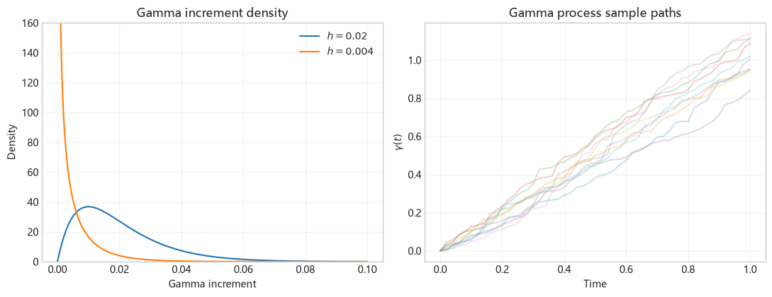
Figure 1.10 Gamma probability densities and sample paths of the Gamma process with parameters \(\mu=1,\nu=0.01,h\in\{1/50,1/250\}\).
1.5.2 Variance Gamma Process
Let \(b(t;\theta,\sigma)=\theta t+\sigma W(t)\) denote Brownian motion with drift rate \(\theta\) and volatility \(\sigma\). In \(b(t)\), we replace calendar time \(t\) by the random time given by \(\gamma(t;1,\nu)\):
\[ X_t(\sigma,\nu,\theta)=b(\gamma(t;1,\nu);\theta,\sigma). \]
This gives the Variance Gamma (VG) process. Among the three parameters of the VG process, \(\theta\) mainly controls the skewness of the distribution, while \(\nu\) mainly controls its kurtosis.
Gamma paths are non-decreasing, so \(G_t=\gamma(t;1,\nu)\) can be interpreted as a business clock. Trading days have the same calendar length, but the amount of information processed by the market, the level of trading activity, and the size of price fluctuations can differ considerably. After a company releases quarterly earnings, for example, the market may process more information in a single day. In the business-clock interpretation, the clock runs faster on that day. More intense market activity corresponds to a greater advance in business time over a fixed calendar interval, while a quiet market corresponds to a smaller advance in business time. This random clock therefore generates stochastic volatility from step to step. For GBM, the standard deviation of each log-return step is \(\sigma\sqrt{h}\); for VG, conditional on the Gamma clock increment \(g\) for that step,
\[ \Delta X\mid\Delta G=g\sim\mathcal{N}(\theta g,\sigma^2g), \qquad \operatorname{SD}(\Delta X_{\mathrm{GBM}})=\sigma\sqrt{h}, \quad \operatorname{SD}(\Delta X_{\mathrm{VG}}\mid\Delta G=g)=\sigma\sqrt{g}. \]
Therefore, over calendar time steps of equal length, GBM has a fixed standard deviation per step, while VG has a conditional standard deviation per step that varies with the Gamma increment. Taking \(h=0.2\), \(\theta=0\), \(\sigma=0.25\), and \(\nu=0.1\) as an example, the table below lists five independent Gamma increments \(\Delta G_i\sim\operatorname{Gamma}(h/\nu,\text{scale}=\nu)=\operatorname{Gamma}(2,0.1)\).
| Time step | \(\Delta G_i\) | GBM standard deviation per step \(\sigma\sqrt{h}\) | VG conditional standard deviation \(\sigma\sqrt{\Delta G_i}\) |
|---|---|---|---|
| 1 | 0.2482 | 0.1118 | 0.1246 |
| 2 | 0.1456 | 0.1118 | 0.0954 |
| 3 | 0.3331 | 0.1118 | 0.1443 |
| 4 | 0.2963 | 0.1118 | 0.1361 |
| 5 | 0.1519 | 0.1118 | 0.0974 |
Table 1.2 Comparison of GBM standard deviation per step and VG conditional standard deviation per step over calendar time steps of equal length.
The VG values in the table are conditional standard deviations given the Gamma increments; averaging over the randomness of the Gamma clock gives the unconditional increment variance \(\operatorname{Var}(\Delta X)=(\sigma^2+\theta^2\nu)h\). In this example, \(\theta=0\), so the unconditional variance remains \(\sigma^2h\).
Let \(X_h=X_{t+h}-X_t\) denote the increment of \(X_t\) over time \(h>0\). The business-clock increment \(G_h\) follows a Gamma distribution with shape parameter \(h/\nu\) and scale parameter \(\nu\). Given \(G_h=g\), \(X_h\) follows a normal distribution with mean \(\theta g\) and variance \(\sigma^2g\). Integrating the conditional normal density against the Gamma density gives the VG increment density:
\[ \begin{aligned} p_h(x) &=\int_0^{+\infty} \frac{1}{\sqrt{2\pi\sigma^2g}} \exp\!\left(-\frac{(x-\theta g)^2}{2\sigma^2g}\right) \frac{g^{h/\nu-1}e^{-g/\nu}} {\nu^{h/\nu}\Gamma(h/\nu)}\,dg. \end{aligned} \]
Evaluating this integral gives the following closed-form density:
\[ \begin{aligned} p_h(x)=\frac{\sqrt{2}e^{\theta x/\sigma^2}} {\sigma\sqrt{\pi}\nu^{h/\nu}\Gamma(h/\nu)} \left(\frac{|x|}{\sqrt{2\sigma^2/\nu+\theta^2}}\right)^{h/\nu-1/2} K_{h/\nu-1/2}\left(\frac{|x|\sqrt{2\sigma^2/\nu+\theta^2}} {\sigma^2}\right). \end{aligned} \tag{1.5.1} \]
Here \(K_v\) denotes the modified Bessel function of the second kind of order \(v\), which solves the modified Bessel ordinary differential equation; the order in equation (1.5.1) is \(v=h/\nu-1/2\).
At \(x=0\), the Bessel expression should be evaluated by taking its limit: the density is finite when \(h/\nu>1/2\); when \(h/\nu\leq1/2\), the density increases without bound, but the singularity is integrable and the distribution still has finite total probability.
The mean and second- through fourth-order central moments of \(X_h\) are, respectively,
\[ \mu_1=E[X_h]=\theta h \tag{1.5.2} \]
\[ \mu_2=E[(X_h-E[X_h])^2]=(\theta^2\nu+\sigma^2)h \tag{1.5.3} \]
\[ \mu_3=E[(X_h-E[X_h])^3]=(2\theta^3\nu^2+3\sigma^2\theta\nu)h \tag{1.5.4} \]
\[ \mu_4=E[(X_h-E[X_h])^4] =(3\sigma^4\nu+12\sigma^2\theta^2\nu^2+6\theta^4\nu^3)h+3\mu_2^2 \tag{1.5.5} \]
The VG process can also be represented as the difference of two independent \(Gamma\) processes. Section 3.2.4.3 introduces this representation.
1.5.3 Moment Estimation for the VG Model
We next fit historical stock returns using the following VG model with drift:
\[ X_t=ct+b(\gamma(t;1,\nu);\theta,\sigma) \tag{1.5.6} \]
Adding the drift term \(ct\) to \(X\) shifts the increment density over \([t,t+h]\). The increment \(X_h=X_{t+h}-X_t\) then has density \(f_h(x)=p_h(x-ch)\) (where \(p_h(\cdot)\) is given by equation (1.5.1)), which can be evaluated using Function 1.5. The function uses the density limit at the center \(x=ch\) and evaluates the Bessel expression elsewhere.
From Formulas to Code
centred corresponds to \(x-ch\), shape to \(h/\nu\), and scale_squared to \(2\sigma^2/\nu+\theta^2\). argument is the argument of the Bessel function.
SciPy’s kve returns \(e^zK_v(z)\), so the code uses \(\log(\operatorname{kve}(v,z))-z\) to calculate \(\log K_v(z)\); \(z\) here is argument.
Function 1.5: Variance Gamma increment density
def variance_gamma_increment_density(
    x, sigma, nu, theta, c, time_step
):
    '''Evaluate the VG increment density at x.

    The parameters are the Brownian volatility sigma, Gamma-clock
    variance rate nu, Brownian drift theta, deterministic drift c,
    and interval length time_step.
    '''
    centred = np.asarray(x, dtype=float) - c * time_step
    shape = time_step / nu
    scale_squared = 2.0 * sigma**2 / nu + theta**2
    absolute_centred = np.where(centred == 0, 1.0, np.abs(centred))
    argument = absolute_centred * np.sqrt(scale_squared) / sigma**2
    power = shape / 2.0 - 0.25
    log_density = (
        np.log(2.0)
        + theta * centred / sigma**2
        - shape * np.log(nu)
        - np.log(sigma)
        - 0.5 * np.log(2.0 * np.pi)
        - gammaln(shape)
        + power
        * (2.0 * np.log(absolute_centred) - np.log(scale_squared))
        + np.log(kve(shape - 0.5, argument))
        - argument
    )
    density = np.exp(log_density)
    if shape > 0.5:
        centre_density = np.exp(
            gammaln(shape - 0.5) - gammaln(shape)
            - np.log(sigma) - 0.5 * np.log(2.0 * np.pi * nu)
            - (shape - 0.5) * np.log(1.0 + theta**2 * nu / (2.0 * sigma**2))
        )
    else:
        centre_density = np.inf  # An integrable density singularity.
    return np.where(centred == 0, centre_density, density)
Figueroa-López et al. (2011) derived moment estimators for the VG process. Adding the drift term \(ct\) changes the first moment of \(X_h\) to
\[ \mu_1=E[X_h]=(\theta+c)h \tag{1.5.7} \]
Since \(c\) is deterministic, adding the drift does not change the second through fourth central moments of \(X_h\). Thus, moment estimation for the VG model in equation (1.5.6) requires solving equations (1.5.3), (1.5.4), (1.5.5), and (1.5.7).
We first calculate the first four sample moments:
\[ \hat\mu_{1,n}=\frac{1}{n}\sum_{i=1}^n x_i=(\hat\theta+\hat c)h \tag{1.5.8} \]
\[ \hat\mu_{k,n}=\frac{1}{n}\sum_{i=1}^n \left(x_i-\hat\mu_{1,n}\right)^k,\quad k=2,3,4 \tag{1.5.9} \]
We then calculate the sample variance, skewness, and kurtosis:
\[ \widehat{Var}_n=\frac{1}{n}\sum_{i=1}^n(x_i-\bar{x})^2 \tag{1.5.10} \]
\[ \widehat{Skw}_n=\frac{\hat\mu_{3,n}}{\hat\mu_{2,n}^{3/2}} \tag{1.5.11} \]
\[ \widehat{Krt}_n=\frac{\hat\mu_{4,n}}{\hat\mu_{2,n}^2}-3 \tag{1.5.12} \]
Define the dimensionless parameter \(\xi=\theta^2\nu/\sigma^2\), which is the ratio of the variance contribution of the random drift in the Gamma clock to that of the Brownian random component. We then solve numerically for its estimate \(\xi^*\), which satisfies
\[ \frac{\xi(3+2\xi)^2}{(1+4\xi+2\xi^2)(1+\xi)} =\frac{3\widehat{Skw}_n^2}{\widehat{Krt}_n} \tag{1.5.13} \]
Substituting this estimate gives the four VG parameter estimates:
\[ \hat\sigma_n^2=\frac{\widehat{Var}_n}{h} \left(\frac{1}{1+\xi^*}\right) \tag{1.5.14} \]
\[ \hat\nu=\frac{h}{3}\widehat{Krt}_n \left(\frac{(1+\xi^*)^2}{1+4\xi^*+2(\xi^*)^2}\right) \tag{1.5.15} \]
\[ \hat\theta=\frac{\hat\mu_{3,n}} {h\hat{\sigma}^2\hat\nu} \left(\frac{1}{3+2\xi^*}\right) \tag{1.5.16} \]
\[ \hat{c}=\frac{1}{h}\bar{x}-\hat\theta =\frac{\sum_{i=1}^n x_i}{T}-\hat\theta \tag{1.5.17} \]
Functions 1.6 calculate the VG moment estimates.
When the sample excess kurtosis satisfies \(\widehat{Krt}_n>0\) and \(0\leq3\widehat{Skw}_n^2/\widehat{Krt}_n<2\), equation (1.5.13) has a unique finite nonnegative solution \(\xi^*\). This follows because the ratio function on the left-hand side is strictly increasing on \(\xi\geq0\), with range \([0,2)\).
# Import the equation solver used in this section
from scipy.optimize import root_scalar
From Formulas to Code
In the ratio function, value corresponds to \(\xi\), and in the moment estimation function, xi_star corresponds to the solution \(\xi^*\). sample_excess_kurtosis stores excess kurtosis, and target corresponds to \(3\widehat{\operatorname{Skew}}^2/\widehat{\operatorname{Kurt}}_{\rm excess}\).
Functions 1.6: Variance Gamma moment ratio and parameter estimation
def vg_moment_ratio(value):
    '''Return the dimensionless VG moment ratio in the xi equation.'''
    return value * (3 + 2 * value) ** 2 / (
        (1 + 4 * value + 2 * value**2) * (1 + value)
    )


def fit_variance_gamma_moments(log_returns, time_step):
    '''Estimate VG parameters from sample moments and cumulants.'''
    sample_mean = np.mean(log_returns)
    sample_variance = np.var(log_returns, ddof=0)
    sample_skewness = skew(log_returns, bias=True)
    sample_excess_kurtosis = kurtosis(
        log_returns, fisher=True, bias=True
    )
    target = 3 * sample_skewness**2 / sample_excess_kurtosis
    root_result = root_scalar(
        lambda value: vg_moment_ratio(value) - target,
        bracket=(0.0, 1.0e6),
        method="brentq",
    )
    xi_star = root_result.root
    sigma = np.sqrt(sample_variance / (time_step * (1 + xi_star)))
    nu = (
        time_step
        / 3
        * sample_excess_kurtosis
        * (1 + xi_star) ** 2
        / (1 + 4 * xi_star + 2 * xi_star**2)
    )
    theta = (
        sample_skewness
        * sample_variance**1.5
        / (time_step * sigma**2 * nu * (3 + 2 * xi_star))
    )
    c = sample_mean / time_step - theta
    return sigma, nu, theta, c
# Use Functions 1.6 to estimate Variance Gamma model parameters
vg_sigma, vg_nu, vg_theta, vg_c = fit_variance_gamma_moments(
log_returns, time_step
)
vg_parameters = pd.Series(
{"sigma": vg_sigma, "nu": vg_nu, "theta": vg_theta, "c": vg_c},
name="VG moment estimates",
)
vg_parameterssigma 0.211462
nu 0.009873
theta -0.075602
c 0.082927
Name: VG moment estimates, dtype: float64# Integrate the VG density over the common bins, using its central singularity as a separate integration breakpoint
vg_hist_edges = fit_bin_edges
vg_bin_centres = fit_bin_centres
vg_bin_counts = model_bin_counts(
lambda x: variance_gamma_increment_density(
x, vg_sigma, vg_nu, vg_theta, vg_c, time_step
), centre=vg_c * time_step
)
vg_expected_counts = vg_bin_counts
vg_normal_counts = normal_bin_countsThe moment estimates for the VG model are
\[ \hat\theta=-0.075602,\quad\hat\nu=0.009873, \quad\hat\sigma=0.211462,\quad\hat c=0.082927 \tag{1.5.18} \]
In Figure 1.11, the red solid line gives the expected count per bin under the VG model, and the blue dashed line gives the corresponding GBM result.
# Figure 1.11: VG fit to daily S&P 500 log returns; VG expected counts in solid red and GBM in dashed blue
fig, ax = plt.subplots(figsize=(8, 4.2))
ax.hist(log_returns, bins=vg_hist_edges, alpha=0.35, label="Sample returns")
ax.plot(
    vg_bin_centres,
    vg_expected_counts,
    color="tab:red",
    label="VG expected counts",
)
ax.plot(
    vg_bin_centres,
    vg_normal_counts,
    color="tab:blue",
    linestyle="--",
    label="GBM expected counts",
)
ax.set_xlim(fit_bin_edges[0], fit_bin_edges[-1])
ax.set_xlabel("Log return")
ax.set_ylabel("Count")
ax.set_title("Variance Gamma fit")
ax.legend()
plt.show()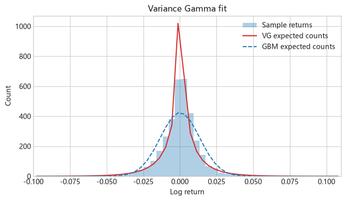
Figure 1.11 VG model fit to S&P 500 index log returns from January 2000 to June 2013. The red solid line gives the expected count per bin for the fitted VG model, and the blue dashed line gives the corresponding GBM result. Both density curves are converted to expected counts for the histogram intervals.
The VG model substantially improves the fit to the tails of the return distribution compared with the normal distribution, but the peak at the center of the distribution is too high.
Figures 1.11a and 1.11b below compare the fits of the VG model and GBM in the left and right tails.
# Figure 1.11a: Compare Variance Gamma and GBM in the left tail
vg_expected_counts = (
    variance_gamma_increment_density(
        tail_return_grid,
        vg_sigma,
        vg_nu,
        vg_theta,
        vg_c,
        time_step,
    )
    * len(log_returns)
    * tail_bin_width
)
plot_tail_comparison(
    tail_return_grid,
    tail_bin_centres,
    histogram_counts,
    tail_bin_width,
    gbm_expected_counts,
    vg_expected_counts,
    "Variance Gamma",
    (log_returns.min(), -0.02),
    "Variance Gamma vs. GBM: left tail",
)
plt.show()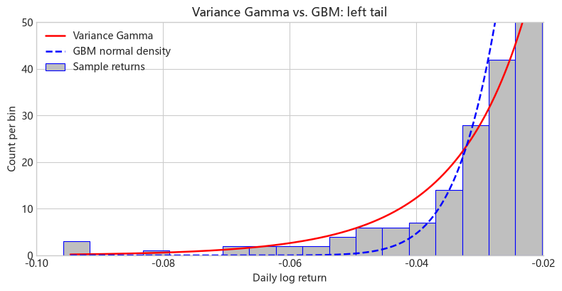
Figure 1.11a Comparison of the Variance Gamma model and GBM in the left tail.
# Figure 1.11b: Compare Variance Gamma and GBM in the right tail
plot_tail_comparison(
    tail_return_grid,
    tail_bin_centres,
    histogram_counts,
    tail_bin_width,
    gbm_expected_counts,
    vg_expected_counts,
    "Variance Gamma",
    (0.02, log_returns.max()),
    "Variance Gamma vs. GBM: right tail",
)
plt.show()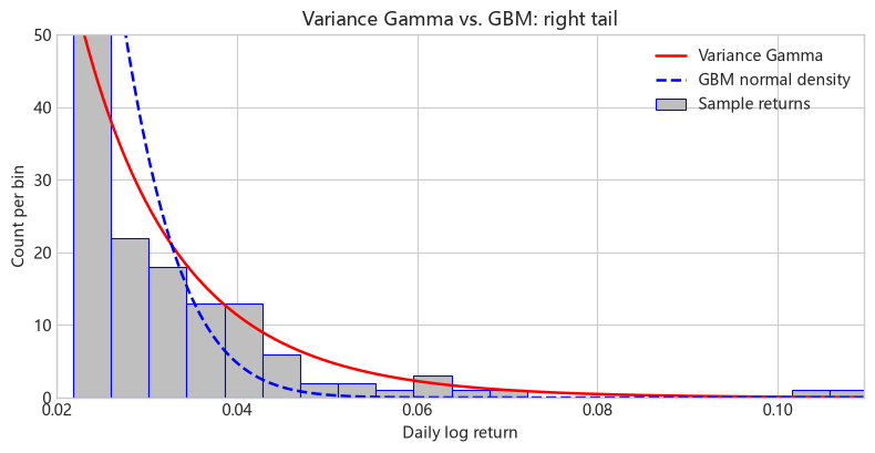
Figure 1.11b Comparison of the Variance Gamma model and GBM in the right tail.
1.6 Normal Inverse Gaussian Model
The Normal Inverse Gaussian (NIG) process was proposed by Barndorff-Nielsen (1997). In this section we fit historical stock returns using the NIG process.
1.6.1 Inverse Gaussian Process
Let \(IG(t;\mu,\lambda)\) denote an inverse Gaussian (IG) process. Over \((t,t+h)\), its increment \(g=IG(t+h;\mu,\lambda)-IG(t;\mu,\lambda)\) follows an inverse Gaussian distribution,
\[ f_h(g;\mu,\lambda)= \sqrt{\frac{\lambda h^2}{2\pi g^3}} \exp\left[-\frac{\lambda(g-\mu h)^2}{2\mu^2g}\right], \quad g>0 \tag{1.6.1} \]
\(\mu>0\) is the mean rate, with increment mean \(E[g]=\mu h\); \(\lambda>0\) is the shape rate, with increment shape parameter \(\lambda h^2\) and variance \(\operatorname{Var}(g)=\mu^3h/\lambda\). When used as the NIG clock in this chapter, \(\mu=1\) and \(\lambda=1/\nu\), so the increment has mean \(h\) and variance \(\nu h\). Below, we calculate the density for \(\mu=1\), \(\nu=0.01\), and \(h\in\{1/50,1/250\}\), and simulate sample paths with \(T=1\).
# Import the numerical, statistical, and plotting libraries used in this section
from scipy.stats import invgauss

inverse_gaussian_mean = 1.0
inverse_gaussian_shape = 1.0 / 0.01
inverse_gaussian_intervals = [1 / 50, 1 / 250]
inverse_gaussian_grid = np.linspace(1e-4, 0.14, 500)
From Formulas to Code
mean_increment corresponds to \(\mu h\), and shape_increment to \(\lambda h^2\). When calling SciPy’s inverse Gaussian density, scipy_shape is their ratio, and shape_increment is passed as the scale parameter.
Function 1.7: Inverse Gaussian increment density
def inverse_gaussian_increment_density(
    increment, mean_rate, shape_rate, interval
):
    '''Evaluate an inverse-Gaussian increment density.

    SciPy's inverse-Gaussian parameter mu is the ratio of the mean
    parameter to the scale parameter, while scale carries the
    interval-dependent shape parameter.
    '''
    mean_increment = mean_rate * interval
    shape_increment = shape_rate * interval**2
    scipy_shape = mean_increment / shape_increment
    return invgauss.pdf(
        increment, mu=scipy_shape, scale=shape_increment
    )
# Figure 1.12, left: Calculate inverse Gaussian increment densities for two time intervals
inverse_gaussian_densities = [
inverse_gaussian_increment_density(
inverse_gaussian_grid,
inverse_gaussian_mean,
inverse_gaussian_shape,
interval,
)
for interval in inverse_gaussian_intervals
]# Figure 1.12, right: Set the time grid for inverse Gaussian process sample paths
inverse_gaussian_path_rng = np.random.default_rng(44)
inverse_gaussian_path_dt = 1 / 50
inverse_gaussian_path_steps = int(1 / inverse_gaussian_path_dt)Function 1.8 generates sample paths by accumulating independent inverse Gaussian increments. Given the number of paths, the number of time steps, and the process parameters, it returns the value of each path at every time point.
From Formulas to Code
NumPy’s rng.wald takes the mean \(\mu h\) and shape parameter \(\lambda h^2\) of the inverse Gaussian distribution as its arguments. increments stores one path’s increments in each row; paths places \(0\) in the first column and then forms cumulative sums along the time axis.
Function 1.8: Simulating inverse Gaussian process paths
def inverse_gaussian_process_paths(
    number_of_paths,
    number_of_steps,
    mean_rate,
    shape_rate,
    time_step,
    rng,
):
    '''Generate inverse-Gaussian-process paths.

    NumPy's wald sampler uses mean=mean_rate*time_step and
    scale=shape_rate*time_step**2 for each increment.
    '''
    increments = rng.wald(
        mean=mean_rate * time_step,
        scale=shape_rate * time_step**2,
        size=(number_of_paths, number_of_steps),
    )
    return np.column_stack(
        [np.zeros(number_of_paths), np.cumsum(increments, axis=1)]
    )
# Figure 1.12, right: Use Function 1.8 to generate ten inverse Gaussian process paths
inverse_gaussian_paths = inverse_gaussian_process_paths(
10,
inverse_gaussian_path_steps,
inverse_gaussian_mean,
inverse_gaussian_shape,
inverse_gaussian_path_dt,
inverse_gaussian_path_rng,
)
inverse_gaussian_path_time = np.linspace(
0.0, 1.0, inverse_gaussian_path_steps + 1
)The left panel of Figure 1.12 shows inverse Gaussian (IG) probability density functions with parameters \(\mu=1,\nu=0.01,h\in\{1/50,1/250\}\). Since IG increments take values in \((0,+\infty)\), the paths of the IG process increase over time, as shown in the right panel of Figure 1.12.
# Figure 1.12: Inverse Gaussian densities (left) and ten process paths (right), with $\mu=1$, $\nu=0.01$, and $h\in\{1/50,1/250\}$
fig, axes = plt.subplots(1, 2, figsize=(11, 4.3))
for interval, density in zip(
    inverse_gaussian_intervals, inverse_gaussian_densities
):
    axes[0].plot(
        inverse_gaussian_grid,
        density,
        label=fr"$h={interval:g}$",
    )
axes[0].set_xlabel("Inverse Gaussian increment")
axes[0].set_ylabel("Density")
axes[0].set_title("Inverse Gaussian increment density")
axes[0].grid(True, alpha=0.25)
axes[0].set_ylim(0.0, 300.0)
axes[0].legend()
axes[1].plot(
    inverse_gaussian_path_time,
    inverse_gaussian_paths.T,
    alpha=0.22,
)
axes[1].set_xlabel("Time")
axes[1].set_ylabel("$IG(t)$")
axes[1].set_title("Inverse Gaussian process sample paths")
axes[1].grid(True, alpha=0.25)
fig.tight_layout()
plt.show()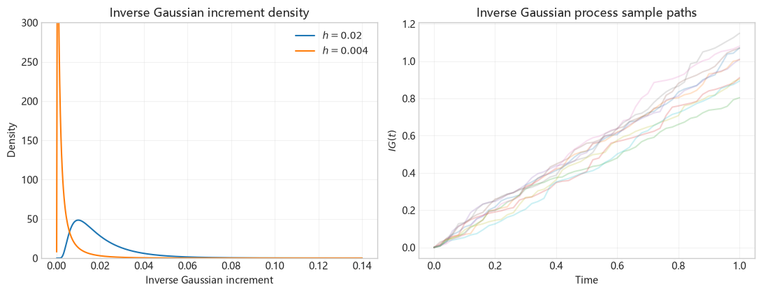
Figure 1.12 Inverse Gaussian densities (left) and 10 sample paths of the inverse Gaussian process (right) for parameters \(\mu=1\), \(\nu=0.01\), and \(h\in\{1/50,1/250\}\).
1.6.2 Normal Inverse Gaussian Process
Assume that Brownian motion and the inverse Gaussian clock are independent. Consider Brownian motion with drift rate \(\theta\) and volatility \(\sigma\), \(b(t;\theta,\sigma)=\theta t+\sigma W(t)\). We replace its calendar time \(t\) by the random time given by \(IG(t;1,1/\nu)\):
\[ X(t;\sigma,\nu,\theta)=b(IG(t;1,1/\nu);\theta,\sigma). \]
This gives the Normal Inverse Gaussian (NIG) process.
NIG and VG use the same time-change construction: Brownian motion runs in business time, and we observe its path in calendar time. NIG uses an inverse Gaussian clock, while VG uses a Gamma clock. If \(H_h=IG(t+h;1,1/\nu)-IG(t;1,1/\nu)\), then given \(H_h=g\), the increment of the basic NIG process also follows \(\mathcal{N}(\theta g,\sigma^2g)\); after adding deterministic drift \(ct\), the conditional mean becomes \(ch+\theta g\). Under this chapter’s parameterization, increments of both clocks have mean \(h\) and variance \(\nu h\), but their distributions differ, so their mixtures of conditional normal distributions also differ, giving rise to different nonnormal return distributions.
Let \(X_h=X_{t+h}-X_t\) denote the increment of \(X_t\) over time \(h>0\). The probability density function of \(X_h\) is given by equation (1.6.2),
\[ \begin{aligned} p_h(x)=\frac{h e^{h/\nu+\theta x/\sigma^2}}{\pi} \left(\frac{x^2+h^2\sigma^2/\nu} {\theta^2/(\nu\sigma^2)+1/\nu^2}\right)^{-1/2} K_1\left(\frac{\sqrt{x^2+h^2\sigma^2/\nu} \sqrt{\sigma^2/\nu+\theta^2}}{\sigma^2}\right). \end{aligned} \tag{1.6.2} \]
and the mean and second- through fourth-order central moments of \(X_h\) are, respectively,
\[ \mu_1=E[X_h]=\theta h \tag{1.6.3} \]
\[ \mu_2=E[(X_h-E[X_h])^2]=(\theta^2\nu+\sigma^2)h \tag{1.6.4} \]
\[ \mu_3=E[(X_h-E[X_h])^3]=(3\theta^3\nu^2+3\sigma^2\theta\nu)h \tag{1.6.5} \]
\[ \mu_4=E[(X_h-E[X_h])^4] =(3\sigma^4\nu+18\sigma^2\theta^2\nu^2+15\theta^4\nu^3)h+3\mu_2^2 \tag{1.6.6} \]
Barndorff-Nielsen (1997) and Schoutens (2003) also give an alternative parameterization of the NIG process. In Section 3.2.5.3 we convert between the two parameterizations.
1.6.2.1 Generalized Moment Estimation for the NIG Process
Next, we use the NIG model with drift
\[ X_t=ct+b(IG(t;1,1/\nu);\theta,\sigma) \tag{1.6.7} \]
to fit the S&P 500 index. After adding the drift term, the increment \(X_h=X_{t+h}-X_t\) of \(X\) over \([t,t+h]\) has density \(f_h(x)=p_h(x-ch)\) (where \(p_h(\cdot)\) is given by equation (1.6.2)), which can be evaluated using Function 1.9a.
In the density function, centred corresponds to \(x-ch\), and alpha, beta, and delta correspond to the transformed parameters. delta already includes the increment length \(h\): \(\delta=\sigma h/\sqrt\nu\). distance corresponds to \(\sqrt{\delta^2+(x-ch)^2}\).
Function 1.9a: Normal inverse Gaussian increment density
def nig_increment_density(x, sigma, nu, theta, c, time_step):
    '''Evaluate the NIG increment density using its Bessel form.'''
    centred = np.asarray(x, dtype=float) - c * time_step
    alpha = np.sqrt(theta**2 + sigma**2 / nu) / sigma**2
    beta = theta / sigma**2
    delta = sigma * time_step / np.sqrt(nu)
    gamma = np.sqrt(alpha**2 - beta**2)
    distance = np.sqrt(delta**2 + centred**2)
    argument = alpha * distance
    log_density = (
        np.log(alpha * delta / np.pi)
        - np.log(distance)
        + delta * gamma
        + beta * centred
        + np.log(kve(1.0, argument))
        - argument
    )
    return np.exp(log_density)
As in the VG model, adding the drift term \(ct\) changes the first moment of \(X_h=X_{t+h}-X_t\) to
\[ \mu_1=E[X_h]=(\theta+c)h \tag{1.6.8} \]
Since \(c\) is deterministic, adding the drift does not change the second through fourth central moments of \(X_h\). Thus, moment estimation for the NIG model in equation (1.6.7) requires solving equations (1.6.4), (1.6.5), (1.6.6), and (1.6.8).
We first calculate the first four sample moments:
\[ \hat\mu_{1,n}=\frac{1}{n}\sum_{i=1}^n x_i=(\hat\theta+\hat c)h \tag{1.6.9} \]
\[ \hat\mu_{k,n}=\frac{1}{n}\sum_{i=1}^n \left(x_i-\hat\mu_{1,n}\right)^k,\quad k=2,3,4 \tag{1.6.10} \]
We then calculate the sample variance, skewness, and kurtosis:
\[ \widehat{\operatorname{Var}}_n=\frac{1}{n} \sum_{i=1}^n(x_i-\bar{x})^2 \tag{1.6.11} \]
\[ \widehat{\operatorname{Skew}}_n=\frac{\hat\mu_{3,n}} {\hat\mu_{2,n}^{3/2}} \tag{1.6.12} \]
\[ \widehat{\operatorname{Kurt}}_{\rm excess,n}=\frac{\hat\mu_{4,n}} {\hat\mu_{2,n}^2}-3 \tag{1.6.13} \]
We again define \(\xi=\theta^2\nu/\sigma^2\), as in the VG model; since the two clocks have different third- and fourth-order cumulants, the formula for its estimate \(\xi^*\) differs:
\[ \xi^*=\frac{\widehat{\operatorname{Skew}}^2} {3\widehat{\operatorname{Kurt}}_{\rm excess} -5\widehat{\operatorname{Skew}}^2} \tag{1.6.14} \]
Substituting this estimate gives the four NIG parameter estimates:
\[ \hat\sigma^2=\frac{\widehat{\operatorname{Var}}_n}{h(1+\xi^*)}, \qquad \hat\sigma_n^2=\hat\sigma^2 \tag{1.6.15} \]
\[ \hat\nu=\frac{h}{3}\widehat{\operatorname{Kurt}}_{\rm excess,n} \frac{1+\xi^*}{1+5\xi^*}, \qquad \hat\nu_n=\hat\nu \tag{1.6.16} \]
\[ \hat\theta_n=\frac{\hat\mu_{3,n}} {h\hat\sigma_n^2\hat\nu_n}\frac{1}{3+3\xi^*} \tag{1.6.17} \]
\[ \hat c=\frac{\widehat\mu_{1,n}}{h}-\hat\theta_n =\frac{1}{h}\bar{x}-\hat\theta_n =\frac{\sum_{i=1}^n x_i}{T}-\hat\theta_n \tag{1.6.18} \]
Function 1.9b calculates the NIG moment estimates.
NIG moment estimation requires positive sample excess kurtosis and \(3\widehat{\operatorname{Kurt}}_{\rm excess}>5\widehat{\operatorname{Skew}}^2\), so that \(\xi^*\) is finite and nonnegative and \(\hat\nu\) is positive.
In the moment estimation function, xi_star corresponds to \(\xi^*\) in equation (1.6.14); the returned sigma, nu, theta, and c correspond to the estimates of the four model parameters.
Function 1.9b: Normal inverse Gaussian parameter estimation from cumulants
def fit_nig_moments(log_returns, time_step):
    '''Estimate NIG parameters from the sample moments.'''
    sample_mean = np.mean(log_returns)
    sample_variance = np.var(log_returns, ddof=0)
    central_moment_3 = np.mean((log_returns - sample_mean) ** 3)
    sample_skewness = skew(log_returns, bias=True)
    sample_excess_kurtosis = kurtosis(
        log_returns, fisher=True, bias=True
    )
    xi_star = sample_skewness**2 / (
        3 * sample_excess_kurtosis - 5 * sample_skewness**2
    )
    sigma = np.sqrt(sample_variance / (time_step * (1 + xi_star)))
    nu = (
        time_step
        / 3
        * sample_excess_kurtosis
        * (1 + xi_star)
        / (1 + 5 * xi_star)
    )
    theta = central_moment_3 / (
        3 * (1 + xi_star) * time_step * sigma**2 * nu
    )
    c = sample_mean / time_step - theta
    return sigma, nu, theta, c
# Use Function 1.9b to estimate NIG model parameters
nig_sigma, nig_nu, nig_theta, nig_c = fit_nig_moments(log_returns, time_step)
nig_parameters = pd.Series(
{"sigma": nig_sigma, "nu": nig_nu, "theta": nig_theta, "c": nig_c},
name="NIG moment estimates",
)
nig_parameterssigma 0.211462
nu 0.009848
theta -0.075761
c 0.083086
Name: NIG moment estimates, dtype: float64The moment estimates for the NIG model are
\[ \hat\sigma=0.211462,\quad\hat\nu=0.009848, \quad\hat\theta=-0.075761,\quad\hat c=0.083086 \tag{1.6.19} \]
Figure 1.13 uses the same bins as the previous three models: the red solid line gives the expected count per bin under the NIG model, and the blue dashed line gives the corresponding GBM result. The quantitative comparison at the end of Section 1.6 provides a further summary of the fit at the center and in the tails.
# Figure 1.13: NIG fit to daily S&P 500 log returns; NIG expected counts in solid red and GBM in dashed blue
nig_grid = fit_bin_centres
nig_bin_counts = model_bin_counts(
    lambda x: nig_increment_density(
        x, nig_sigma, nig_nu, nig_theta, nig_c, time_step
    )
)
fig, ax = plt.subplots(figsize=(8, 4.2))
ax.hist(log_returns, bins=fit_bin_edges, alpha=0.35, label="Sample returns")
ax.plot(
    nig_grid,
    nig_bin_counts,
    color="tab:red",
    label="NIG expected counts",
)
ax.plot(
    nig_grid,
    normal_bin_counts,
    color="tab:blue",
    linestyle="--",
    label="GBM expected counts",
)
ax.set_xlim(fit_bin_edges[0], fit_bin_edges[-1])
ax.set_xlabel("Log return")
ax.set_ylabel("Count")
ax.set_title("Normal Inverse Gaussian fit")
ax.legend()
plt.show()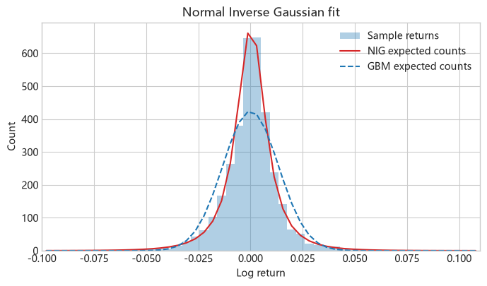
Figure 1.13 NIG model fit to S&P 500 index log returns from January 2000 to June 2013. The red solid line gives the expected count per bin for the fitted NIG model, and the blue dashed line gives the corresponding GBM result. Model counts in the overall plot are calculated by integrating the density over each bin.
The NIG model appears to provide the best fit to both the tails and the peak among the four models considered in this section.
We next compare the fits of the NIG model and GBM in the left and right tails.
# Figure 1.13a: Compare Normal Inverse Gaussian and GBM in the left tail
nig_expected_counts = (
    nig_increment_density(
        tail_return_grid,
        nig_sigma,
        nig_nu,
        nig_theta,
        nig_c,
        time_step,
    )
    * len(log_returns)
    * tail_bin_width
)
plot_tail_comparison(
    tail_return_grid,
    tail_bin_centres,
    histogram_counts,
    tail_bin_width,
    gbm_expected_counts,
    nig_expected_counts,
    "Normal Inverse Gaussian",
    (log_returns.min(), -0.02),
    "Normal Inverse Gaussian vs. GBM: left tail",
)
plt.show()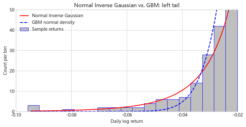
Figure 1.13a Comparison of the Normal Inverse Gaussian model and GBM in the left tail.
# Figure 1.13b: Compare Normal Inverse Gaussian and GBM in the right tail
plot_tail_comparison(
    tail_return_grid,
    tail_bin_centres,
    histogram_counts,
    tail_bin_width,
    gbm_expected_counts,
    nig_expected_counts,
    "Normal Inverse Gaussian",
    (0.02, log_returns.max()),
    "Normal Inverse Gaussian vs. GBM: right tail",
)
plt.show()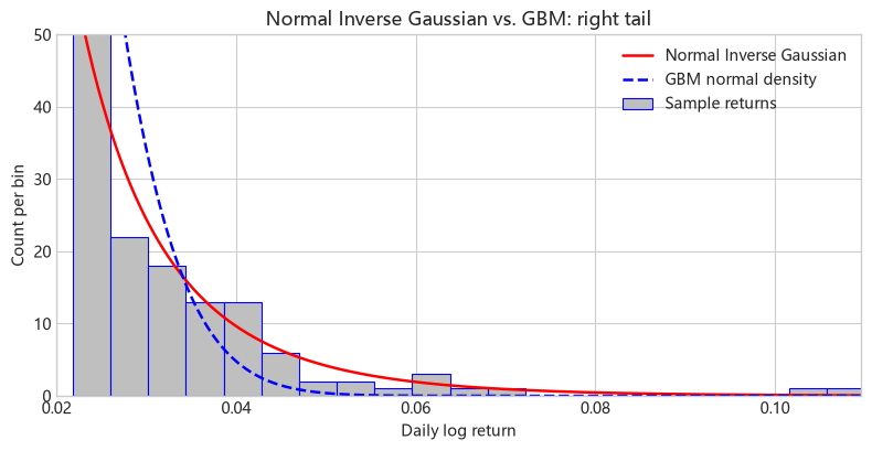
Figure 1.13b Comparison of the Normal Inverse Gaussian model and GBM in the right tail.
Comparison of In-Sample Fits of the Four Models
The average log-likelihood per observation is \(n^{-1}\sum_i\log f(x_i)\); a larger value indicates that the model assigns a higher overall density to the observed returns. The binned total variation is \(\frac12\sum_j|\widehat p_j-p_j|\); a smaller value indicates that the model frequencies are closer to the sample frequencies. The calculation includes probabilities beyond both ends of the plotting interval. We calculate tail probabilities at two daily log-return thresholds, \(a\in\{3\%,4\%\}\): the left-tail probability is \(P(X<-a)\) and the right-tail probability is \(P(X>a)\). Each probability can be compared directly with the corresponding sample proportion.
# Table 1.4: Compare the four models on the same historical sample
fitted_densities = {
    "GBM": lambda x: norm.pdf(x, loc=sample_mean, scale=np.sqrt(sample_variance)),
    "Merton": lambda x: merton_increment_density(
        x, merton_drift, merton_diffusion_volatility,
        merton_jump_intensity, 0.0, merton_jump_std, time_step),
    "VG": lambda x: variance_gamma_increment_density(
        x, vg_sigma, vg_nu, vg_theta, vg_c, time_step),
    "NIG": lambda x: nig_increment_density(
        x, nig_sigma, nig_nu, nig_theta, nig_c, time_step),
}
fitted_bin_counts = {
    "GBM": normal_bin_counts, "Merton": merton_bin_counts,
    "VG": vg_bin_counts, "NIG": nig_bin_counts,
}
observed_counts, _ = np.histogram(log_returns, bins=fit_bin_edges)
observed_probabilities = np.r_[
    np.mean(log_returns < fit_bin_edges[0]),
    observed_counts / len(log_returns),
    np.mean(log_returns > fit_bin_edges[-1]),
]
comparison_rows = []
for model_name, density in fitted_densities.items():
    left_outside = quad(density, -np.inf, fit_bin_edges[0])[0]
    right_outside = quad(density, fit_bin_edges[-1], np.inf)[0]
    probabilities = np.r_[left_outside,
                          fitted_bin_counts[model_name] / len(log_returns),
                          right_outside]
    comparison_rows.append({
        "Model": model_name,
        "Average log-likelihood (higher is better)": np.mean(np.log(density(log_returns))),
        "Binned total variation": 0.5 * np.sum(np.abs(observed_probabilities - probabilities)),
        "Left-tail probability (below -3%)": quad(density, -np.inf, -0.03)[0],
        "Right-tail probability (above 3%)": quad(density, 0.03, np.inf)[0],
        "Left-tail probability (below -4%)": quad(density, -np.inf, -0.04)[0],
        "Right-tail probability (above 4%)": quad(density, 0.04, np.inf)[0],
    })
fit_comparison = pd.DataFrame(comparison_rows).set_index("Model")
fit_comparison.loc["Sample", :] = [np.nan, np.nan,
    np.mean(log_returns < -0.03), np.mean(log_returns > 0.03),
    np.mean(log_returns < -0.04), np.mean(log_returns > 0.04)]
fit_comparison| Average log-likelihood (higher is better) | Binned total variation | Left-tail probability (below -3%) | Right-tail probability (above 3%) | Left-tail probability (below -4%) | Right-tail probability (above 4%) | |
|---|---|---|---|---|---|---|
| Model | ||||||
| GBM | 2.897977 | 0.165333 | 0.012196 | 0.012335 | 0.001348 | 0.001367 |
| Merton | 2.999307 | 0.100533 | 0.014816 | 0.014874 | 0.008601 | 0.008626 |
| VG | 2.958058 | 0.130640 | 0.024674 | 0.022531 | 0.011307 | 0.009952 |
| NIG | 3.022572 | 0.040682 | 0.021384 | 0.019559 | 0.009691 | 0.008496 |
| Sample | NaN | NaN | 0.019458 | 0.018278 | 0.008550 | 0.007370 |
Table 1.4 Fit measures using the same sample and bins.
Conclusions from the comparison.
- NIG gives the best overall fit, followed by Merton, VG, and GBM. Both overall measures give the same ranking. NIG has the highest average log-likelihood, 3.0226, and the smallest binned total variation, 0.0407; the corresponding GBM values are 2.8980 and 0.1653. All three models with jumps improve the overall fit relative to GBM.
- GBM underestimates the probabilities of returns beyond \(\pm3\%\) and \(\pm4\%\). At the 3% threshold, GBM gives left- and right-tail probabilities of 1.22% and 1.23%, compared with sample proportions of 1.95% and 1.83%. At the 4% threshold, the GBM probabilities fall to 0.135% and 0.137%, while the sample proportions remain 0.855% and 0.737%. These results quantify the normal distribution’s underestimation of extreme return probabilities.
- NIG gives the closest left- and right-tail probabilities at the 3% threshold; at 4%, Merton is closest in the left tail and NIG in the right tail. NIG gives probabilities of 2.14% and 1.96% at the 3% threshold. At 4%, Merton gives a left-tail probability of 0.860%, close to the sample proportion of 0.855%; NIG gives a right-tail probability of 0.850%, close to the sample proportion of 0.737%. NIG therefore gives the best overall fit, while Merton also closely matches the observed frequency of returns below -4%.
1.7 Risk-Neutral Pricing
1.7.1 The Risk-Neutral World
Risk-neutral pricing was proposed by Cox and Ross (1976). Under the risk-neutral measure, an asset’s expected rate of return equals the risk-free rate. We price the asset by discounting its expected future cash flows at this rate. Denoting the risk-neutral measure by \(Q\), the expected stock price at a future time \(t>0\) is
\[E^Q[S_t]=S_0e^{rt}.\]
If the dynamics of the underlying asset \(S\) in the risk-neutral world are known, any European option on \(S\) can be priced using equation (1.7.1):
\[V_t(S)=e^{-r(T-t)}E^Q[V_T\mid S_t=S]\tag{1.7.1}.\]
This is the risk-neutral pricing formula for European options.
Risk-neutral pricing is justified by replication and no arbitrage: when an option payoff can be replicated by trading in the stock and a risk-free asset, the option price equals the cost of the replicating portfolio. Section 4.1 derives the Black–Scholes–Merton PDE by Delta hedging and then uses the Feynman–Kac formula to express its solution as the risk-neutral discounted expectation in equation (1.7.1).
The advantage of risk-neutral pricing is that risk adjustment is incorporated into the probability distribution under \(Q\), while cash flows are discounted at the same risk-free rate \(r\). Once the risk-neutral model is specified, we calculate the expected payoff and discount it. This removes the need to estimate the underlying asset’s expected return in the real world or to choose a separate risk-adjusted discount rate for each option.
For example, in the GBM model without dividends, the risk-neutral log drift is \(r-\sigma^2/2\), determined by the risk-free rate and volatility. We can therefore calculate a European option price from the current stock price, strike, remaining maturity, risk-free rate, and volatility. This gives the numerical methods in later chapters a specific computational task: calculate the expected option payoff under the specified risk-neutral distribution.
Next, we adjust the deterministic drift of each of the four log-return processes so that the stock satisfies \(E^Q[S_t]=S_0e^{rt}\).
1.7.1.1 Determining Risk-Neutral Drift Using the Moment-Generating Function
We first write the log price as
\[S_t=S_0e^{X_t},\quad X_t=c_Qt+Y_t,\]
where \(Y_t\) is the random component with stationary independent increments, and \(c_Q\) denotes the deterministic drift inside the exponent in the risk-neutral world. The discounted stock price must satisfy
\[E^Q[e^{-rt}S_t]=S_0.\]
We substitute \(S_t\) and divide by \(S_0\) to obtain
\[e^{-rt}e^{c_Qt}E^Q[e^{Y_t}]=1.\]
We denote the moment-generating function of \(Y_t\) by \(M_{Y_t}(u)=E^Q[e^{uY_t}]\) and its cumulant-generating function by \(K_{Y_t}(u)=\log M_{Y_t}(u)\). Then
\[e^{c_Qt}M_{Y_t}(1)=e^{rt},\quad c_Q=r-\frac{K_{Y_t}(1)}{t}.\]
This gives the general formula for the risk-neutral drift: first calculate \(K_{Y_t}(1)\) for the risk-neutral random component, then subtract its contribution per unit time, \(K_{Y_t}(1)/t\), from \(r\).
1.7.1.2 Geometric Brownian Motion
In the risk-neutral world, we write the random component as \(Y_t=\sigma W_t\). Its moment-generating and cumulant-generating functions are, respectively,
\[ M_{Y_t}(u)=E^Q[e^{uY_t}]=e^{\sigma^2u^2t/2}, \qquad K_{Y_t}(u)=\log M_{Y_t}(u)=\frac{1}{2}\sigma^2u^2t. \]
Substituting \(u=1\) into the general formula \(c_Q=r-K_{Y_t}(1)/t\) gives
\[ c_Q^{GBM}=r-\frac{1}{2}\sigma^2. \]
Thus the risk-neutral GBM is
\[ S_t=S_0\exp\left((r-\tfrac12\sigma^2)t+\sigma W_t\right), \quad W_t\sim N(0,t), \]
or, equivalently,
\[ X_t\sim N\left((r-\sigma^2/2)t,\sigma^2t\right). \]
For maturity \(T\), it can also be written as
\[ S_T=S_0\exp\left((r-\tfrac12\sigma^2)T+\sigma\sqrt{T}Z\right), \quad Z\sim N(0,1). \]
1.7.1.3 Merton Jump Diffusion Process
In the risk-neutral world, we write the random component as \(Y_t=\sigma W_t+\sum_{i=1}^{N_t}J_i\), where \(N_t\sim\operatorname{Poisson}(\lambda t)\) and \(J_i\sim N(a,b^2)\). Conditional on \(N_t=n\), the moment-generating function of the total jump component is
\[ E^Q\left[e^{u\sum_{i=1}^{N_t}J_i}\mid N_t=n\right] =\left(M_J(u)\right)^n, \qquad M_J(u)=E^Q[e^{uJ_1}]. \]
Taking the expectation over the Poisson jump count gives
\[ \begin{aligned} E^Q\left[e^{u\sum_{i=1}^{N_t}J_i}\right] &=\sum_{n=0}^{\infty}\left(M_J(u)\right)^n \frac{e^{-\lambda t}(\lambda t)^n}{n!}\\ &=\exp\left(\lambda t\left[M_J(u)-1\right]\right). \end{aligned} \]
Using the independence of the Brownian and jump components, the moment-generating and cumulant-generating functions of the random component are
\[ \begin{aligned} M_{Y_t}(u) &=\exp\left\{t\left(\frac{\sigma^2u^2}{2} +\lambda[M_J(u)-1]\right)\right\},\\ K_{Y_t}(u) &=\log M_{Y_t}(u) =t\left(\frac{\sigma^2u^2}{2} +\lambda[M_J(u)-1]\right). \end{aligned} \]
Since \(J_1\sim N(a,b^2)\), we have
\[ M_J(u)=e^{au+b^2u^2/2}, \qquad M_J(1)=e^{a+b^2/2}. \]
From the general formula \(c_Q=r-K_{Y_t}(1)/t\), the total risk-neutral log drift of the Merton model is
\[ c_Q^{JD}=r-\frac{\sigma^2}{2} -\lambda\left(e^{a+b^2/2}-1\right). \]
If we denote the additional correction for jumps by \(q_{JD}=-\lambda[M_J(1)-1]\), this can be written as
\[ q_{JD}=-\lambda\left(e^{a+b^2/2}-1\right), \qquad c_Q^{JD}=r-\frac{\sigma^2}{2}+q_{JD}. \]
1.7.1.4 Exponential VG Process
For the exponential VG process, let \(G_t=\gamma(t;1,\nu)\); the random component is
\[ Y_t=\theta G_t+\sigma W_{G_t}. \]
We first condition on the value of the business clock, \(G_t=g\). Then \(W_g\sim N(0,g)\) and \(Y_t\mid G_t=g=\theta g+\sigma W_g\). Using the moment-generating function of a normal random variable, \(E[e^{sW_g}]=e^{s^2g/2}\), gives
\[ \begin{aligned} E^Q[e^{uY_t}\mid G_t=g] &=e^{u\theta g}E^Q[e^{u\sigma W_g}]\\ &=e^{u\theta g+\sigma^2u^2g/2} =e^{v(u)g},\\ v(u)&=u\theta+\frac{1}{2}\sigma^2u^2. \end{aligned} \]
We then average over the random clock using the law of total expectation:
\[ M_{Y_t}(u)=E^Q[e^{uY_t}] =E^Q\!\left[E^Q[e^{uY_t}\mid G_t]\right] =E^Q[e^{v(u)G_t}]. \]
Thus, the moment-generating function of \(Y_t\) is the moment-generating function of the Gamma clock evaluated at \(v=v(u)\). Here \(G_t\sim\operatorname{Gamma}(k,\text{scale}=\nu)\), where \(k=t/\nu\), and its density is
\[ f_{G_t}(g)=\frac{g^{k-1}e^{-g/\nu}}{\nu^k\Gamma(k)},\quad g>0. \]
We calculate the moment-generating function of the clock by direct integration. For \(v<1/\nu\), let \(a=1/\nu-v>0\) and use the Gamma integral \(\int_0^\infty g^{k-1}e^{-ag}\,dg=\Gamma(k)a^{-k}\):
\[ \begin{aligned} E^Q[e^{vG_t}] &=\frac{1}{\nu^k\Gamma(k)} \int_0^\infty g^{k-1}e^{-(1/\nu-v)g}\,dg\\ &=\frac{\Gamma(k)(1/\nu-v)^{-k}} {\nu^k\Gamma(k)} =(1-\nu v)^{-k}. \end{aligned} \]
Substituting \(k=t/\nu\) and \(v(u)=u\theta+\sigma^2u^2/2\) gives the moment-generating function of the VG random component; taking its logarithm gives the cumulant-generating function:
\[ \begin{aligned} M_{Y_t}(u) &=\left(1-\theta\nu u-\frac{\sigma^2\nu u^2}{2}\right)^{-t/\nu},\\ K_{Y_t}(u) &=\log M_{Y_t}(u) =-\frac{t}{\nu}\log\left(1-\theta\nu u -\frac{\sigma^2\nu u^2}{2}\right). \end{aligned} \]
From \(c_Q=r-K_{Y_t}(1)/t\), we have
\[ q_{VG}=-\frac{K_{Y_t}(1)}{t} =\frac{1}{\nu}\log\left(1-\theta\nu-\frac{\sigma^2\nu}{2}\right), \qquad c_Q^{VG}=r+q_{VG}. \]
Thus the risk-neutral exponential VG process can be written as
\[ S_t=S_0\exp\left((r+q_{VG})t+Y_t\right). \]
For parameters satisfying \(1-\theta\nu-\sigma^2\nu/2>0\), \(M_{Y_t}(1)\) is finite, and substituting the compensation term above gives \(E^Q[S_t]=S_0e^{rt}\).
1.7.1.5 Exponential NIG Process
For the exponential NIG process, let \(G_t=IG(t;1,1/\nu)\); the random component is
\[ Y_t=\theta G_t+\sigma W_{G_t}. \]
VG and NIG have the same conditional normal component. Given \(G_t=g\), we have \(Y_t\mid G_t=g\sim N(\theta g,\sigma^2g)\), so let
\[ v(u)=u\theta+\frac{1}{2}\sigma^2u^2, \qquad M_{Y_t}(u)=E^Q[e^{v(u)G_t}]. \]
The difference lies in the clock: NIG uses an inverse Gaussian business clock. Under the parameterization in this chapter, \(G_t\) has mean \(t\) and variance \(\nu t\), and its density is
\[ f_{G_t}(g)=\frac{t}{\sqrt{2\pi\nu g^3}} \exp\left(-\frac{(g-t)^2}{2\nu g}\right),\quad g>0. \]
We substitute the density into the moment-generating function of the clock and collect the terms in the exponent:
\[ \begin{aligned} E^Q[e^{vG_t}] &=\frac{t e^{t/\nu}}{\sqrt{2\pi\nu}} \int_0^\infty g^{-3/2} \exp\left[-\frac{1-2\nu v}{2\nu}g -\frac{t^2}{2\nu g}\right]dg. \end{aligned} \]
We use the integral identity
\[ \int_0^\infty g^{-3/2}e^{-Ag-B/g}\,dg =\sqrt{\frac{\pi}{B}}e^{-2\sqrt{AB}},\quad A,B>0, \]
where \(A=(1-2\nu v)/(2\nu)\) and \(B=t^2/(2\nu)\). Simplifying gives the moment-generating function of the inverse Gaussian clock
\[ E^Q[e^{vG_t}] =\exp\left[\frac{t}{\nu} \left(1-\sqrt{1-2\nu v}\right)\right], \quad v<\frac{1}{2\nu}. \]
At the boundary \(v=1/(2\nu)\), \(A=0\) in the integral; the integral still converges, and the MGF equals \(e^{t/\nu}\). Thus the expression above can be extended continuously to this boundary.
Substituting \(v(u)=u\theta+\sigma^2u^2/2\) into \(M_{Y_t}(u)=E^Q[e^{v(u)G_t}]\) and then taking the logarithm gives the moment-generating and cumulant-generating functions of the NIG random component:
\[ \begin{aligned} M_{Y_t}(u) &=\exp\left\{\frac{t}{\nu} \left(1-\sqrt{1-2\theta\nu u-\sigma^2\nu u^2}\right)\right\},\\ K_{Y_t}(u) &=\log M_{Y_t}(u) =\frac{t}{\nu} \left(1-\sqrt{1-2\theta\nu u-\sigma^2\nu u^2}\right). \end{aligned} \]
From \(c_Q=r-K_{Y_t}(1)/t\), we obtain
\[ q_{NIG}=-\frac{K_{Y_t}(1)}{t} =-\frac{1}{\nu}\left(1-\sqrt{1-2\theta\nu-\sigma^2\nu}\right), \qquad c_Q^{NIG}=r+q_{NIG}. \]
The NIG MGF is finite when the expression under the square root is nonnegative, so the condition at \(u=1\) is \(1-2\theta\nu-\sigma^2\nu\geq0\). At the boundary, \(M_{Y_t}(1)=e^{t/\nu}\). Differentiating the MGF introduces a factor \((1-2\theta\nu u-\sigma^2\nu u^2)^{-1/2}\), so we calculate derivatives within the parameter range where the expression under the square root is strictly positive.
For VG and NIG, both compensation terms satisfy \(q=-K_{Y_t}(1)/t\), so
\[ e^{-qt}=E^Q[e^{Y_t}]=M_{Y_t}(1)=e^{K_{Y_t}(1)}. \]
This agrees with the general formula \(c_Q=r-K_{Y_t}(1)/t\); the definitions and properties of moment-generating and cumulant-generating functions will be discussed further in Chapter 5.
In this section, \(q\) denotes the risk-neutral compensation term in the log-price process. The drift \(c\) in historical fitting is determined by the sample mean: \(\hat c=\bar x/h-\hat\theta\); the risk-neutral drift is determined by \(c_Q=r-K_{Y_t}(1)/t\). The former matches the mean of historical returns, while the latter matches the risk-neutral expected growth rate of the stock.
Table 1.3 summarises the drift rates of the various stochastic processes in the risk-neutral world.
| Distribution | Parameters | Log drift rate in the risk-neutral world |
|---|---|---|
| Brownian motion | \((\mu,\sigma)\) | \(r-\sigma^2/2\) |
| Merton jump diffusion | \((\mu,\sigma,\lambda,a,b)\) | \(r-\sigma^2/2-\lambda(e^{a+b^2/2}-1)\) |
| VG | \((\theta,\sigma,\nu)\) | \(r+\nu^{-1}\log(1-\theta\nu-\sigma^2\nu/2)\) |
| NIG | \((\theta,\sigma,\nu)\) | \(r-\nu^{-1}(1-\sqrt{1-2\theta\nu-\sigma^2\nu})\) |
Table 1.3 Drift rates of various stochastic processes in the risk-neutral world
1.8 The Black–Scholes Formula
The Black–Scholes–Merton (BSM) model assumes that stock prices follow geometric Brownian motion. The option price is determined by the following factors:
- Current price of the underlying asset \(S_0\);
- Volatility of the underlying asset \(\sigma\);
- Option strike price \(K\);
- Option maturity \(T\);
- Risk-free interest rate \(r\).
The model also makes the following assumptions:
- Investors can lend and borrow money at the market risk-free interest rate;
- The underlying asset pays no dividends;
- Transaction costs are zero, and there is no bid–ask spread;
- Shares are divisible, and investors can hold or sell short any quantity.
Black and Scholes (1973) derived an analytical expression for European stock option prices. Known as the Black–Scholes formula, it is the most widely used option pricing formula.
Under risk-neutral pricing, we consider an option with maturity \(T\) and underlying asset \(S\). If the stock price \(S_T=S_0e^{X_T}\) follows geometric Brownian motion, then
\[ X_T\sim N\left((r-\sigma^2/2)T,\sigma^2T\right). \]
For a call option, we first calculate the expected payoff at maturity:
\[ \begin{aligned} E^Q[(S_T-K)^+] &=E^Q[(S_0e^{X_T}-K)^+]\\ &=\int_{\log(K/S_0)}^{+\infty}(S_0e^x-K) \frac{1}{\sqrt{2\pi\sigma^2T}} \exp\left[-\frac{(x-(r-\sigma^2/2)T)^2}{2\sigma^2T}\right]dx. \end{aligned} \]
We change variables from \([x-(r-\sigma^2/2)T]/(\sigma\sqrt T)\) to \(y\) and define
\[ y=\frac{x-(r-\sigma^2/2)T}{\sigma\sqrt T},\quad a=\frac{\log(K/S_0)-(r-\sigma^2/2)T}{\sigma\sqrt T}=-d_2. \]
Replacing \([x-(r-\sigma^2/2)T]/(\sigma\sqrt T)\) by \(y\) gives
\[ \begin{aligned} E^Q[(S_T-K)^+] =&\int_a^{+\infty} \left(S_0e^{\sigma\sqrt T y+(r-\sigma^2/2)T}-K\right)\phi(y)\,dy\\ =&S_0e^{rT}\int_a^{+\infty} e^{\sigma\sqrt T y-\sigma^2T/2}\phi(y)\,dy -K\int_a^{+\infty}\phi(y)\,dy. \end{aligned} \]
The integral in the second term above is a standard normal tail probability; the first term also becomes a standard normal tail probability after the substitution \(z=y-\sigma\sqrt T\). Using the standard normal density \(\phi\), we can write the second term as
\[ K\Phi\left(\frac{\log(S_0/K)+(r-\sigma^2/2)T} {\sigma\sqrt T}\right). \]
where \(\Phi\) denotes the standard normal distribution function. The first term also becomes a standard normal tail probability after the substitution \(z=y-\sigma\sqrt T\), so it can be written as
\[ S_0e^{rT}\Phi\left(\frac{\log(S_0/K)+(r+\sigma^2/2)T} {\sigma\sqrt T}\right). \]
Since the price of a European call option at \(t\) is \(C(S,t)=e^{-r(T-t)}E^Q[(S_T-K)^+\mid S_t=S]\), the derivation above gives the following expression for \(C(S,t)\):
\[ C(S,t)=S\Phi(d_1)-Ke^{-r(T-t)}\Phi(d_2) \tag{1.8.1} \]
where
\[ d_1=\frac{\log(S/K)+(r+\sigma^2/2)(T-t)} {\sigma\sqrt{T-t}} \tag{1.8.2} \]
\[ d_2=d_1-\sigma\sqrt{T-t} \tag{1.8.3} \]
The two terms in the call option formula also have intuitive meanings. In the BSM model without dividends, \(\Phi(d_2)\) is the risk-neutral probability that the stock price at maturity exceeds the strike price. Thus \(Ke^{-r(T-t)}\Phi(d_2)\) is the expected present value of the strike payment, and \(S\Phi(d_1)\) is the expected present value of the stock received on exercise. \(d_2\) comes from the threshold in the exercise condition \(S_T>K\). To calculate the expected stock component, we also weight each exercise scenario by the terminal stock price \(S_T\): a higher stock price makes a larger contribution to this term. This weighting changes the argument of the normal distribution function to \(d_1=d_2+\sigma\sqrt{T-t}\), which explains why the two terms use different values of the normal distribution function.
This is the Black–Scholes formula. We can derive the European put price in the same way or obtain it from put–call parity.
1.8.1 Put–Call Parity
Let \(\omega\) represent any possible scenario at \(T\) for a European option. By the definitions of call and put options, their discounted payoffs at maturity in this scenario are, respectively,
\[ \widetilde g_C(\omega)=e^{-rT}(S_T(\omega)-K)^+, \quad \widetilde g_P(\omega)=e^{-rT}(K-S_T(\omega))^+. \]
Whether \(S_T(\omega)\geq K\) or \(S_T(\omega)<K\), the discounted payoffs satisfy the following identity:
\[ \widetilde g_C(\omega)-\widetilde g_P(\omega)=e^{-rT}(S_T(\omega)-K). \]
Taking the expectation of both sides gives put–call parity:
\[ C-P=e^{-rT}E^Q[S_T-K]=S_0-e^{-rT}K \tag{1.8.4} \]
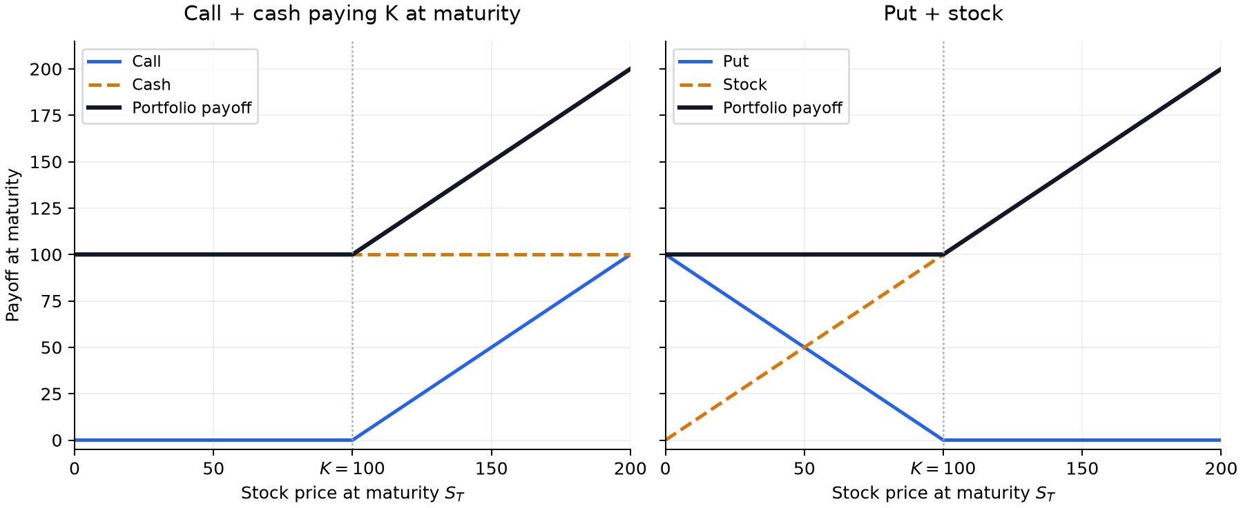
Illustration of Put–Call Parity (\(K=100\)). The left portfolio holds a call and cash that pays \(K\) at maturity; the right holds a put and the stock. Both pay \(\max(S_T,K)\), so their current costs satisfy \(C+Ke^{-rT}=P+S_0\).
In the BSM model, substituting the call option pricing formula (1.8.1) gives
\[ \begin{aligned} P(S,t)&=C(S,t)+Ke^{-r(T-t)}-S\\ &=Ke^{-r(T-t)}\Phi(-d_2)-S\Phi(-d_1) \end{aligned} \tag{1.8.5} \]
The European call and put option prices above can be calculated using Functions 1.10.
# Define the fixed parameters for the BSM example
S0 = 100.0
K = 100.0
T = 1.0
r = 0.05
sigma = 0.20
From Formulas to Code
d1 and d2 correspond to \(d_1,d_2\) in the pricing formula; T denotes the remaining time to maturity. discount corresponds to \(e^{-rT}\), and norm.cdf calculates the standard normal distribution function \(\Phi\).
Functions 1.10: Black–Scholes intermediate quantities and call and put prices (cp=1 denotes a call, cp=-1 denotes a put)
def black_scholes_d1_d2(sigma, S0, K, T, r):
    """Return the two standardized distances used in the BSM formula."""
    d1 = (np.log(S0 / K) + (r + sigma**2 / 2) * T) / (sigma * np.sqrt(T))
    d2 = d1 - sigma * np.sqrt(T)
    return d1, d2


def black_scholes_formula(sigma, S0, K, T, r, cp):
    """Return a no-dividend European call (cp=1) or put (cp=-1) value."""
    if cp not in (-1, 1):
        raise ValueError("cp must be 1 for a call or -1 for a put")
    d1, d2 = black_scholes_d1_d2(sigma, S0, K, T, r)
    discount = np.exp(-r * T)
    return cp * (S0 * norm.cdf(cp * d1) - K * discount * norm.cdf(cp * d2))


# The first five arguments follow def black_scholes_formula(sigma, S0, K, T, r); cp is the sixth argument.
# Organize the inputs to Functions 1.10 using model and option objects
from quant_option_pricing import BlackScholesModel, EuropeanOption
model = BlackScholesModel(rate=r, volatility=sigma)
call_option = EuropeanOption.call(spot=S0, strike=K, maturity=T)
put_option = EuropeanOption.put(spot=S0, strike=K, maturity=T)
d1, d2 = black_scholes_d1_d2(
model.volatility,
call_option.spot,
call_option.strike,
call_option.maturity,
model.rate,
)
call_value = black_scholes_formula(
model.volatility,
call_option.spot,
call_option.strike,
call_option.maturity,
model.rate,
call_option.cp,
)
put_value = black_scholes_formula(
model.volatility,
put_option.spot,
put_option.strike,
put_option.maturity,
model.rate,
put_option.cp,
)
pd.Series({"d1": d1, "d2": d2, "Call option": call_value, "Put option": put_value})d1 0.350000
d2 0.150000
Call option 10.450584
Put option 5.573526
dtype: float641.9 Greeks
Option sensitivity parameters, also called Greeks, measure the response of the option price to changes in variables or parameters. They are used to measure and manage option risk.
1.9.1 Delta
The most important sensitivity parameter is Delta. Delta measures the change in the option price when the underlying asset price changes, that is,
\[ \Delta=\frac{\partial V}{\partial S} \tag{1.9.1} \]
Holding time fixed, we expand the option price \(V\) in a Taylor series around the current stock price \(S_0\) to obtain
\[ V(S) \approx V(S_0) + \dfrac{\partial V}{\partial S}(S-S_0) +\dfrac{1}{2}\dfrac{\partial^2 V}{\partial S^2}(S-S_0)^2 \tag{1.9.2} \]
If the underlying asset price changes only slightly, the second-order derivative term can be neglected, and equation (1.9.2) simplifies to
\[ V(S) - V(S_0) = \Delta(S-S_0). \]
Holding 1 option and \(-\Delta\) shares of the underlying asset gives a first-order stock price sensitivity of \(\Delta-\Delta=0\), so, to first order, the portfolio value remains constant at
\[ V(S)-\Delta S = V(S_0)-\Delta S_0. \]
This portfolio is therefore called a Delta-neutral portfolio.
Delta is a function of the asset price, so a price change also changes Delta. To keep the portfolio Delta-neutral, the stock holding per option must be adjusted to match the new Delta.
1.9.2 Gamma
Gamma measures the sensitivity of Delta to the underlying asset price,
\[ \Gamma = \dfrac{\partial \Delta}{\partial S} = \dfrac{\partial^2 V}{\partial S^2} \tag{1.9.3} \]
When the stock price changes by a small amount \(\delta S\), the change in Delta is approximately \(\Gamma\,\delta S\). For an option hedged with \(-\Delta\) shares, restoring Delta neutrality requires adjusting the stock position by approximately \(-\Gamma\,\delta S\) shares. Thus, for the same stock price change, a larger absolute Gamma requires a larger adjustment to the hedge position.
We can also write the Taylor expansion of the option price as
\[ V(S)-V(S_0)\approx \Delta(S-S_0)+\dfrac{1}{2}\Gamma(S-S_0)^2. \tag{1.9.4} \]
This is the Delta-Gamma estimate of the option price change resulting from a change in the underlying asset price. It is the second-order Taylor expansion of \(V(S)\) around \(S_0\) and can be applied to price scenarios generated by normal return models and the leptokurtic, heavy-tailed return models introduced earlier. If the stock position remains at \(-\Delta\), first-order changes cancel, and the second-order portfolio value change is approximately \(\tfrac12\Gamma(S-S_0)^2\).
1.9.3 Theta
Theta measures the effect of changes in time on the theoretical value of an option.
\[ \Theta = \dfrac{\partial V_t}{\partial t} \tag{1.9.5} \]
Theta represents the local effect of the passage of calendar time on the option price, holding the underlying price and other parameters fixed. Time is measured in years, and we take \(h=1/250\) for one trading day. Over this interval the price change is approximately \(\Theta h\); negative Theta corresponds to a decrease in value, while positive Theta corresponds to an increase.
Adding a Theta term to equation (1.9.4) gives the Delta-Gamma-Theta estimate of the option price.
\[ V(S,t)-V(S_0,t_0)\approx \Theta(t-t_0)+\Delta(S-S_0) +\dfrac{1}{2}\Gamma(S-S_0)^2. \tag{1.9.6} \]
1.9.4 Vega
Vega measures the change in the option price when the volatility of the underlying asset price changes,
\[ \nu = \dfrac{\partial V}{\partial \sigma}. \tag{1.9.7} \]
European put and call options always have equal Vega. Using put–call parity \(C-P=S_0-Ke^{-rT}=S_0-e^{-rT}K\), we differentiate both sides with respect to volatility to obtain
\[ \dfrac{\partial}{\partial \sigma}(C-P)=\nu_C-\nu_P \tag{1.9.8} \]
\[ \dfrac{\partial}{\partial \sigma}(S_0-e^{-rT}K)=0. \tag{1.9.9} \]
Thus \(\nu_C-\nu_P=0\), that is, \(\nu_C=\nu_P\). Here we use Vega to denote this sensitivity parameter to avoid confusion with the time-change parameter \(\nu\) in the VG and NIG models. Call and put option Vegas are equal and positive.
1.9.5 Rho
Rho describes the sensitivity of the option price to changes in the risk-free interest rate,
\[ \rho=\dfrac{\partial V_t}{\partial r} \tag{1.9.10} \]
An interest rate change \(\delta r\) gives an approximate price change of \(\rho\,\delta r\). For options on a stock that pays no dividends, the BSM formulas below give \(|\rho|\leq K\tau e^{-r\tau}\), where \(\tau=T-t\); as the remaining time to maturity decreases, this upper bound on interest rate sensitivity decreases toward zero in proportion to \(\tau\). For example, with Rho equal to 20, an interest rate increase of one percentage point gives an approximate price change of \(20\times0.01=0.20\).
1.9.6 Greeks in the BSM Model
We first give the expressions for the call option Greeks in the BSM model.
\[ \Delta_C=\Phi(d_1) \tag{1.9.11} \]
\[ \Gamma_C=\dfrac{\phi(d_1)}{S\sigma\sqrt{T-t}} \tag{1.9.12} \]
\[ \nu_C=S\phi(d_1)\sqrt{T-t} =Ke^{-r(T-t)}\phi(d_2)\sqrt{T-t} \tag{1.9.13} \]
\[ \Theta_C=-\dfrac{S\phi(d_1)\sigma}{2\sqrt{T-t}} -rKe^{-r(T-t)}\Phi(d_2) \tag{1.9.14} \]
\[ \rho_C=K(T-t)e^{-r(T-t)}\Phi(d_2) \tag{1.9.15} \]
In the BSM model without dividends, with \(S,K,\sigma,T-t>0\) and \(r\geq0\), call option Delta, Gamma, Vega, and Rho are positive, while Theta is negative.
The put option Greeks are
\[ \Delta_P=-\Phi(-d_1)=\Delta_C-1 \tag{1.9.16} \]
\[ \Gamma_P=\Gamma_C \tag{1.9.17} \]
\[ \nu_P=\nu_C \tag{1.9.18} \]
\[ \Theta_P=-\dfrac{S\phi(-d_1)\sigma}{2\sqrt{T-t}} +rKe^{-r(T-t)}\Phi(-d_2)=\Theta_C+rKe^{-r(T-t)} \tag{1.9.19} \]
\[ \rho_P=-K(T-t)e^{-r(T-t)}\Phi(-d_2) \tag{1.9.20} \]
We next derive Delta, Gamma, and Vega for a call option. The derivation uses the following two identities:
\[ \dfrac{\partial \Phi(d_1)}{\partial d_1}=\phi(d_1) \tag{1.9.21} \]
\[ \dfrac{\partial \Phi(d_2)}{\partial d_2}=\phi(d_2) =\phi(d_1)e^{d_1\sigma\sqrt{T-t}}e^{-\frac{\sigma^2(T-t)}{2}} =\phi(d_1)S_te^{r(T-t)}/K. \tag{1.9.22} \]
Differentiating equation (1.8.1) with respect to \(S_t\) gives
\[ \begin{aligned} \Delta_C&=\Phi(d_1)+S_t\dfrac{\partial \Phi(d_1)}{\partial S_t} -Ke^{-r(T-t)}\dfrac{\partial \Phi(d_2)}{\partial S_t}\\ &=\Phi(d_1)+S_t\dfrac{\partial \Phi(d_1)}{\partial d_1} \dfrac{\partial d_1}{\partial S_t} -Ke^{-r(T-t)}\dfrac{\partial \Phi(d_2)}{\partial d_2} \dfrac{\partial d_2}{\partial S_t}\\ &=\Phi(d_1)+S_t\phi(d_1)\dfrac{1}{S_t\sigma\sqrt{T-t}} -Ke^{-r(T-t)}\phi(d_1)\dfrac{S_te^{r(T-t)}}{K} \dfrac{1}{S_t\sigma\sqrt{T-t}}\\ &=\Phi(d_1). \end{aligned} \]
where \(\partial d_1/\partial S_t=\partial d_2/\partial S_t=1/(S_t\sigma\sqrt{T-t})\), and we have used equation (1.9.22).
Differentiating Delta with respect to \(S_t\) gives
\[ \Gamma_C=\dfrac{\partial \Delta_C}{\partial S_t} =\dfrac{\partial \Phi(d_1)}{\partial d_1} \dfrac{\partial d_1}{\partial S_t} =\dfrac{\phi(d_1)}{S_t\sigma\sqrt{T-t}}. \]
Differentiating equation (1.8.1) with respect to \(\sigma\) gives
\[ \begin{aligned} \nu_C&=S_t\dfrac{\partial \Phi(d_1)}{\partial \sigma} -Ke^{-r(T-t)}\dfrac{\partial \Phi(d_2)}{\partial \sigma}\\ &=S_t\dfrac{\partial \Phi(d_1)}{\partial d_1} \dfrac{\partial d_1}{\partial \sigma} -Ke^{-r(T-t)}\dfrac{\partial \Phi(d_2)}{\partial d_2} \dfrac{\partial d_2}{\partial \sigma}. \end{aligned} \]
Differentiating \(d_1\) and \(d_2\) with respect to \(\sigma\), respectively, gives
\[ \begin{aligned} \dfrac{\partial d_1}{\partial \sigma} &=\dfrac{\sigma^2(T-t)^{3/2} -\left[\log\left(S/K\right)+\left(r+\sigma^2/2\right)(T-t)\right]\sqrt{T-t}} {\sigma^2(T-t)}\\ \dfrac{\partial d_2}{\partial \sigma} &=\dfrac{-\left[\log\left(S/K\right)+\left(r+\sigma^2/2\right)(T-t)\right]\sqrt{T-t}} {\sigma^2(T-t)}. \end{aligned} \]
Therefore
\[ \nu_C=S\phi(d_1)\sqrt{T-t} =Ke^{-r(T-t)}\phi(d_2)\sqrt{T-t}. \tag{1.9.23} \]
From Formulas to Code
density corresponds to the standard normal density \(\phi(d_1)\), and discount corresponds to \(e^{-rT}\). In the returned dictionary, delta, gamma, vega, theta, and rho store the respective sensitivity parameters.
Functions 1.11: Black–Scholes call and put Greeks
def call_greeks_formula(sigma, S0, K, T, r):
    '''Return Delta, Gamma, Vega, Theta, and Rho for a call.'''
    d1 = (np.log(S0 / K) + (r + sigma**2 / 2) * T) / (sigma * np.sqrt(T))
    d2 = d1 - sigma * np.sqrt(T)
    density = norm.pdf(d1)
    discount = np.exp(-r * T)
    return {
        "delta": norm.cdf(d1),
        "gamma": density / (S0 * sigma * np.sqrt(T)),
        "vega": S0 * density * np.sqrt(T),
        "theta": -S0 * density * sigma / (2 * np.sqrt(T))
        - r * K * discount * norm.cdf(d2),
        "rho": K * T * discount * norm.cdf(d2),
    }

def put_greeks_formula(sigma, S0, K, T, r):
    '''Return Delta, Gamma, Vega, Theta, and Rho for a put.'''
    d1 = (np.log(S0 / K) + (r + sigma**2 / 2) * T) / (sigma * np.sqrt(T))
    d2 = d1 - sigma * np.sqrt(T)
    density = norm.pdf(d1)
    discount = np.exp(-r * T)
    return {
        "delta": norm.cdf(d1) - 1.0,
        "gamma": density / (S0 * sigma * np.sqrt(T)),
        "vega": S0 * density * np.sqrt(T),
        "theta": -S0 * density * sigma / (2 * np.sqrt(T))
        + r * K * discount * norm.cdf(-d2),
        "rho": -K * T * discount * norm.cdf(-d2),
    }
# Use Functions 1.11 to calculate call and put Greeks
call_greeks = call_greeks_formula(sigma, S0, K, T, r)
put_greeks = put_greeks_formula(sigma, S0, K, T, r)
pd.DataFrame({"Call": call_greeks, "Put": put_greeks})| Call | Put | |
|---|---|---|
| delta | 0.636831 | -0.363169 |
| gamma | 0.018762 | 0.018762 |
| vega | 37.524035 | 37.524035 |
| theta | -6.414028 | -1.657880 |
| rho | 53.232482 | -41.890461 |
Figure 1.14 shows BSM prices, Delta, Gamma, Vega, and Theta for European call and put options with current stock prices \(0<S_0\leq40\) and maturities of \(T=0.1\) year and \(T=1\) year. The other parameters are \(\sigma=0.2\), \(K=20\), and \(r=5\%\). Below, \(S\) denotes the current stock price and \(\tau=T-t\) the remaining time to maturity; the plots use \(t=0\), so \(\tau=T\). The plots illustrate the following properties of the BSM Greeks:
- European call Delta lies in \((0,1)\), while European put Delta lies in \((-1,0)\). Delta increases with the underlying asset price.
- European call and put Gammas are equal and positive. Differentiating equation (1.9.12) with respect to \(S\) shows that Gamma peaks at \(d_1=-\sigma\sqrt\tau\), corresponding to \(S_\Gamma^*=K\exp[-(r+3\sigma^2/2)\tau]\); Gamma decreases as the stock price moves away from this peak in either direction. Holding \(K,r,\sigma\) fixed, consider the behavior as the remaining time \(\tau\) decreases toward zero. When the option is at the money, \(S=K\), Gamma is approximately \(1/(K\sigma\sqrt{2\pi\tau})\) and increases as the remaining time decreases. At any fixed stock price below or above \(K\), Gamma decreases toward zero as expiry approaches. Near maturity, the option price curve approaches a straight line on each side of the strike, with its curvature concentrated in an increasingly narrow region around \(K\). Thus the Gamma peak rises while Gamma away from the strike falls.
- European call and put Vegas are equal and positive. Differentiating equation (1.9.13) with respect to \(S\) gives a peak at \(d_1=\sigma\sqrt\tau\), corresponding to \(S_{\mathrm{Vega}}^*=K\exp[(\sigma^2/2-r)\tau]\); Vega decreases as the stock price moves away from this peak in either direction. Holding \(K,r,\sigma\) fixed, Vega decreases toward zero as expiry approaches for every fixed stock price \(S>0\), including the at-the-money point \(S=K\). At-the-money Vega is approximately \(K\sqrt{\tau/(2\pi)}\), so it decreases in proportion to the square root of the remaining time. As the remaining time decreases, a change in volatility has a smaller effect on the terminal stock price distribution; at maturity, the payoff is determined directly by the stock price and strike. Consequently, the Vega peak falls as maturity approaches, whereas the Gamma peak rises.
- With no dividends and \(r\geq0\), European call Theta is negative. Put Theta is the sum of the diffusion term \(-S\sigma\phi(d_1)/(2\sqrt\tau)\) and the interest term \(rKe^{-r\tau}\Phi(-d_2)\). As \(S\to0\) with \(r>0\), the former approaches zero and Theta approaches \(rKe^{-r\tau}>0\). Near maturity, the leading term for both at-the-money call and put Theta is \(-K\sigma/(2\sqrt{2\pi\tau})\), so the loss of time value accelerates. As \(\tau\to0\) with the stock price fixed, call Theta approaches \(-rK\) for \(S>K\) and zero for \(S<K\); put Theta approaches \(rK\) for \(S<K\) and zero for \(S>K\).
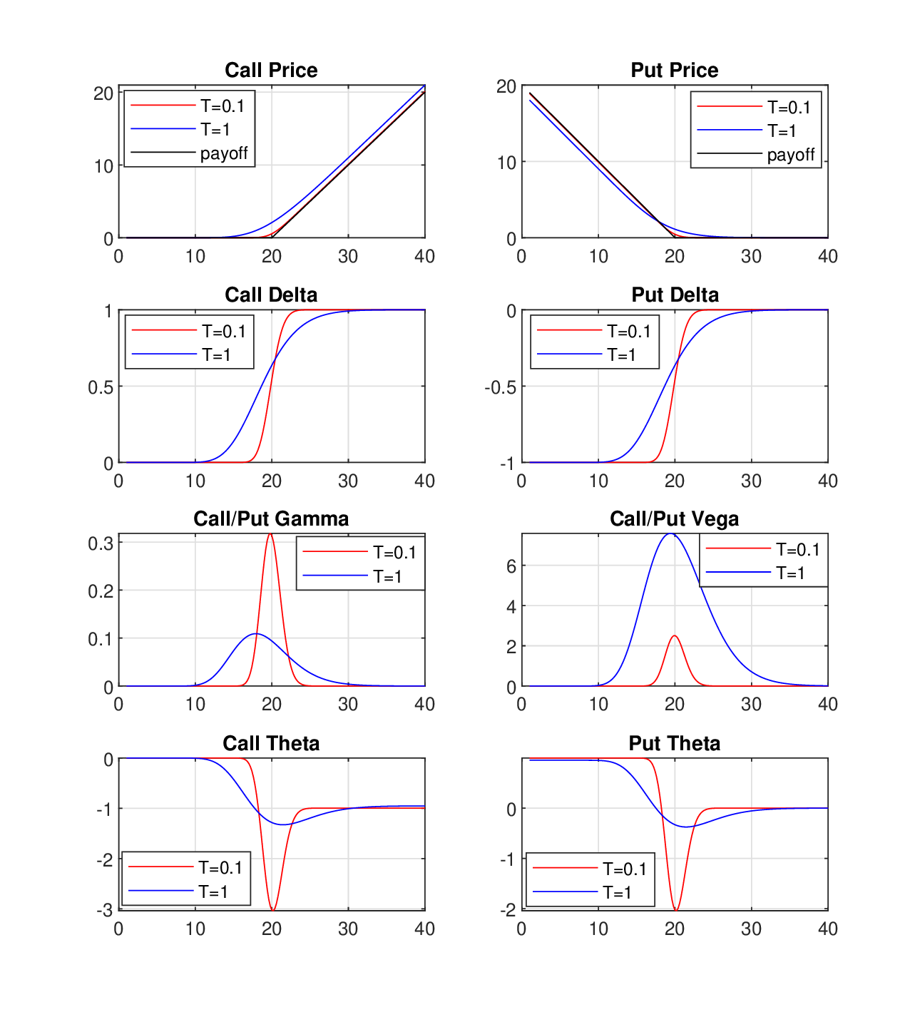
Figure 1.14 Prices and Greeks of European call and put options in the Black–Scholes model, where \(0<S_0\leq40\), \(T\in\{0.1,1\}\), \(\sigma=0.2\), \(K=20\), and \(r=5\%\).
1.9.7 Delta-Gamma-Theta Estimation under the BSM Model
We previously introduced the Delta-Gamma-Theta approximation to the option price:
\[ V(S,t)-V(S_0,t_0)\approx \Theta(t-t_0)+\Delta(S-S_0) +\dfrac{1}{2}\Gamma(S-S_0)^2. \tag{1.9.24} \]
Delta-Gamma-Theta estimation is widely used to measure and manage risk in portfolios containing options or other financial derivatives. Managing the risk of a trading portfolio often requires estimating its profit and loss distribution over a future risk horizon, for example to calculate Value at Risk. To obtain the distribution of portfolio values, we could generate many scenarios for the asset price \(S\) by Monte Carlo simulation and reprice the option in each scenario. If no analytical formula is available for the option price but Delta, Gamma, and Theta are known, this estimate avoids numerical repricing in every scenario and saves considerable time. We use the same initial Delta, Gamma, and Theta in all scenarios, so each scenario requires evaluating only the three terms in equation (1.9.24).
We next compare the Delta-Gamma-Theta estimate with Black–Scholes prices. We first calculate Delta, Gamma, and Theta under the Black–Scholes model. We then consider daily returns within \(\pm10\%\) on the stock \(S\), reprice the option using the Black–Scholes formula, and compare the resulting prices with the Delta-Gamma-Theta estimates.
# Figure 1.15: Set option parameters and calculate the initial price and Greeks
dgt_spot = 100.0
dgt_strike = 120.0
dgt_maturity = 1.0
dgt_rate = 0.05
dgt_volatility = 0.20
dgt_greeks = call_greeks_formula(
    dgt_volatility, dgt_spot, dgt_strike, dgt_maturity, dgt_rate
)
dgt_initial_value = black_scholes_formula(
    dgt_volatility, dgt_spot, dgt_strike, dgt_maturity, dgt_rate, cp=1
)
dgt_greeks
{'delta': np.float64(0.28719163790512714),
'gamma': np.float64(0.017036921138505086),
'vega': np.float64(34.07384227701017),
'theta': np.float64(-4.680968546398613),
'rho': np.float64(25.4716863739519)}# Figure 1.15: Calculate exact price changes and the Delta-Gamma-Theta approximation
dgt_time_step = 1.0 / 250.0
dgt_price_changes = dgt_spot * np.arange(-0.10, 0.101, 0.01)
dgt_exact_changes = np.array(
[
black_scholes_formula(
dgt_volatility,
dgt_spot + price_change,
dgt_strike,
dgt_maturity - dgt_time_step,
dgt_rate,
1,
)
- dgt_initial_value
for price_change in dgt_price_changes
]
)
approx_change = (
dgt_greeks["theta"] * dgt_time_step
+ dgt_greeks["delta"] * dgt_price_changes
+ 0.5 * dgt_greeks["gamma"] * dgt_price_changes**2
)
pd.DataFrame(
{
"Stock price change": dgt_price_changes,
"Exact change": dgt_exact_changes,
"Delta-Gamma-Theta approximation": approx_change,
}
).head()| Stock price change | Exact change | Delta-Gamma-Theta approximation | |
|---|---|---|---|
| 0 | -10.0 | -2.096989 | -2.038794 |
| 1 | -9.0 | -1.953354 | -1.913453 |
| 2 | -8.0 | -1.796886 | -1.771076 |
| 3 | -7.0 | -1.627005 | -1.611661 |
| 4 | -6.0 | -1.443150 | -1.435209 |
# Figure 1.15: Delta-Gamma-Theta approximation of option value under Black-Scholes
fig, ax = plt.subplots(figsize=(8, 4.2))
ax.plot(dgt_price_changes, dgt_exact_changes, "o-", label="Exact BSM repricing")
ax.plot(dgt_price_changes, approx_change, "--", label="Delta–Gamma–Theta approximation")
ax.set_xlabel("Stock price change")
ax.set_ylabel("Option value change")
ax.set_title("Delta–Gamma–Theta approximation")
ax.legend(frameon=False)
ax.grid(True, alpha=0.25)
fig.tight_layout()
plt.show()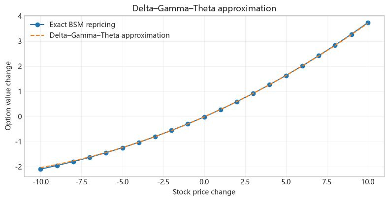
Figure 1.15 Delta–Gamma–Theta approximation of option value under the Black–Scholes model.
In Figure 1.15, the Delta–Gamma–Theta approximation closely matches exact BSM repricing over the interval of one trading day and the stock price changes within \(\pm10\%\) considered in this example. The positive Gamma term captures the upward curvature by adding a positive quadratic adjustment for both stock price rises and falls. With the stock price unchanged, the estimated value change is \(\Theta/250\), representing the loss of time value over one trading day. Thus the three Greeks calculated at the initial point accurately approximate the option value changes across the price scenarios shown.
1.10 Implied Volatility
In the Black–Scholes model, the option price is determined by the following factors:
- Current price of the underlying asset \(S_0\);
- Volatility of the underlying asset \(\sigma\);
- Option strike price \(K\);
- Option maturity \(T\);
- Risk-free interest rate \(r\).
With \(S_0,K,T,r\) known, volatility determines the option price. Conversely, we can solve for volatility from the option price. Section 1.3.1 introduced volatility estimation from historical stock prices. The resulting estimate is called historical volatility. However, pricing options with historical volatility usually produces theoretical prices that differ substantially from market option prices. In practice, volatility is usually inferred from option prices. This is called implied volatility: the volatility obtained by inverting an option pricing model at the observed market price (premium). It reflects the market’s expectation of the asset’s future return. Substituting an option’s implied volatility into the pricing model gives its market price:
\[ \sigma_{\mathrm{imp}}: V(\sigma_{\mathrm{imp}},S_0,K,T,r)=V_{\mathrm{market}}. \]
Since option Vega \(>0\), the higher the volatility of the underlying asset, the higher the European option price. Figure 1.16 shows that European call option prices in the BSM model increase with volatility \(\sigma\). When \(S_0,K,T>0\) and the market price lies strictly between the price bounds in Section 1.10.1, there is a unique, finite, positive implied volatility.
# Figure 1.16: Set option parameters and calculate prices across volatility values
iv_spot = 100.0
iv_strike = 120.0
iv_maturity = 1.0
iv_rate = 0.05
iv_cp = 1
iv_market_price = 2.0

volatility_values = np.linspace(0.01, 0.80, 250)
volatility_prices = np.array(
    [
        black_scholes_formula(
            volatility,
            iv_spot,
            iv_strike,
            iv_maturity,
            iv_rate,
            iv_cp,
        )
        for volatility in volatility_values
    ]
)
# Figure 1.16: Black-Scholes call value versus volatility, with $S_0=100$, $r=5\%$, $T=1$, and $K=120$
fig, ax = plt.subplots(figsize=(8, 4.2))
ax.plot(volatility_values, volatility_prices)
ax.set_xlabel("Volatility")
ax.set_ylabel("Call value")
ax.set_title("Call value versus volatility")
ax.grid(True, alpha=0.25)
fig.tight_layout()
plt.show()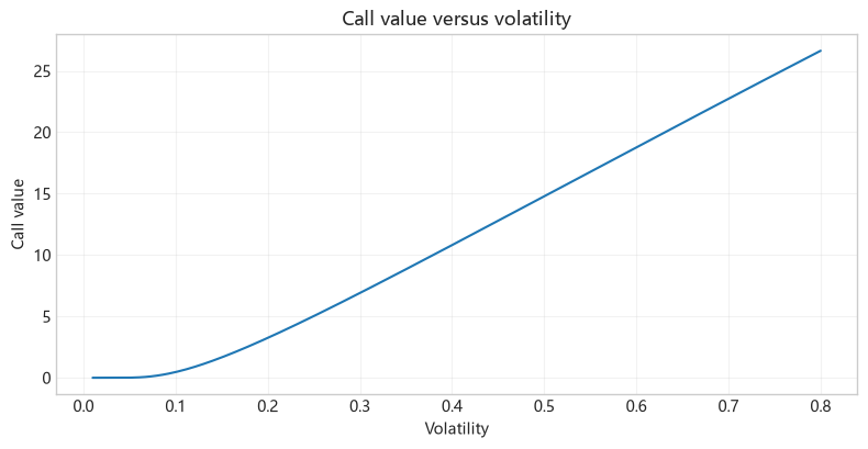
Figure 1.16 Black–Scholes European call option value as a function of volatility, where \(S_0=100\), \(r=5\%\), \(T=1\), and \(K=120\).
1.10.1 Solving for Implied Volatility Numerically
In general, implied volatility must be calculated numerically. For example, Function 1.12 uses bisection. At each iteration, the sign of the price error determines which half of the current interval contains the solution. Define
\[ f(\sigma)=V(\sigma,S_0,K,T,r)-V_{\mathrm{market}}. \]
For a European call option without dividends, the market price must satisfy
\[ \max(S_0-Ke^{-rT},0)\leq V_{\mathrm{market}}\leq S_0. \]
The corresponding condition for a put option is
\[ \max(Ke^{-rT}-S_0,0)\leq P_{\mathrm{market}}\leq Ke^{-rT}. \]
When the no-arbitrage bounds are satisfied, the price errors at the endpoints of the initial bisection interval must have opposite signs, that is, \(f(\sigma_{\mathrm{low}})f(\sigma_{\mathrm{high}})\leq0\). We start with a sufficiently wide interval and calculate its midpoint at each iteration: if the model price at the midpoint is higher than the market price, move the upper bound to the midpoint; if the model price is lower than the market price, move the lower bound to the midpoint. Each iteration halves the interval width; after \(m\) iterations, its width is \(2^{-m}\) times the initial width, and the distance from the midpoint to the root within the interval is at most half this width.
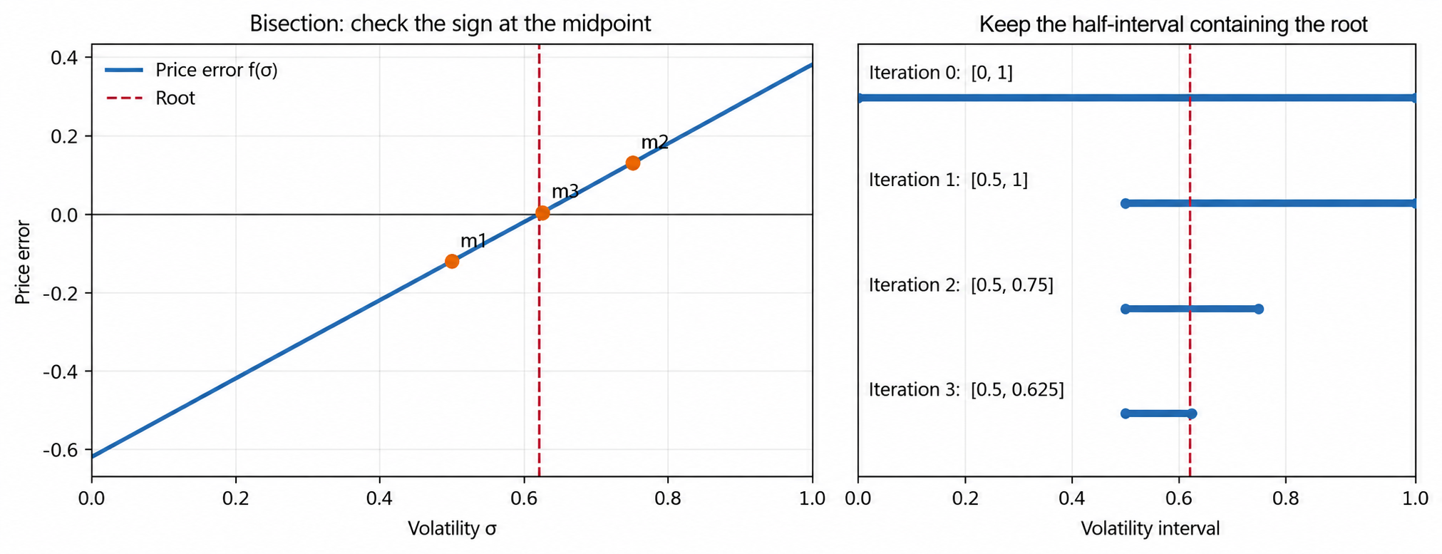
Schematic of the bisection method. The left panel shows how the sign of the price error at the midpoint determines which half of the interval contains the root. The right panel shows the intervals narrowing as this step is repeated.
From Formulas to Code
target is the market option price, low and high are the two endpoints of the volatility search interval, and mid is the interval midpoint. error corresponds to the value of \(f(\sigma)=V_{\rm BS}(\sigma)-V_{\rm market}\) at the midpoint; its sign is used to choose the interval for the next iteration.
Function 1.12: Implied volatility by bisection
def implied_volatility_bisection(
    target, S0, K, T, r, cp, low=1e-8, high=5.0
):
    if low <= 0 or high <= low:
        raise ValueError("Volatility interval must satisfy 0 < low < high")
    low_error = black_scholes_formula(low, S0, K, T, r, cp) - target
    high_error = black_scholes_formula(high, S0, K, T, r, cp) - target
    if low_error * high_error > 0:
        raise ValueError("Market price lies outside the specified volatility interval")
    # Bisection returns implied volatility and the iteration history
    iteration_rows = []
    for iteration in range(100):
        mid = 0.5 * (low + high)
        error = black_scholes_formula(mid, S0, K, T, r, cp) - target
        iteration_rows.append(
            {
                "Iteration": iteration,
                "Volatility lower bound": low,
                "Volatility upper bound": high,
                "Midpoint": mid,
                "Price error": error,
            }
        )
        if abs(error) < 1e-10:
            return mid, pd.DataFrame(iteration_rows)
        if error > 0:
            high = mid
        else:
            low = mid
    return 0.5 * (low + high), pd.DataFrame(iteration_rows)
# Function 1.12 example: Solve for implied volatility and display bisection iterations
target_price = iv_market_price
bisection_volatility, bisection_iterations = implied_volatility_bisection(
target_price,
iv_spot,
iv_strike,
iv_maturity,
iv_rate,
iv_cp,
)
bisection_iterations.head(8)| Iteration | Volatility lower bound | Volatility upper bound | Midpoint | Price error | |
|---|---|---|---|---|---|
| 0 | 0 | 1.000000e-08 | 5.000000 | 2.500000 | 75.443706 |
| 1 | 1 | 1.000000e-08 | 2.500000 | 1.250000 | 41.285267 |
| 2 | 2 | 1.000000e-08 | 1.250000 | 0.625000 | 17.762321 |
| 3 | 3 | 1.000000e-08 | 0.625000 | 0.312500 | 5.383629 |
| 4 | 4 | 1.000000e-08 | 0.312500 | 0.156250 | -0.157154 |
| 5 | 5 | 1.562500e-01 | 0.312500 | 0.234375 | 2.456042 |
| 6 | 6 | 1.562500e-01 | 0.234375 | 0.195313 | 1.088574 |
| 7 | 7 | 1.562500e-01 | 0.195313 | 0.175781 | 0.446166 |
Bisection result. For this example, bisection gives
\[ \sigma_{\mathrm{imp}}^{\mathrm{(bisect)}}\approx 0.161483, \]
that is, an implied volatility of approximately \(16.15\%\). Using this volatility in the BSM call option pricing function gives a price of approximately \(2\), consistent with the given market price.
1.10.2 Vega and Implied Volatility
Vega, the derivative of the option price with respect to volatility, \(\partial V/\partial\sigma\), has an analytical expression in the Black–Scholes model. We can use it in Newton iterations to solve for implied volatility more efficiently. In Section 1.9.6, we derived the analytical expression (1.9.23) for \(\nu=\partial V/\partial\sigma\), which we now use to solve for implied volatility. Function 1.13 implements the Newton iteration:
\[ \sigma_{m+1}=\sigma_m-\frac{V(\sigma_m)-V_{\mathrm{market}}}{\operatorname{Vega}(\sigma_m)}. \]
Newton’s method divides the price error \(\delta V\) by Vega to calculate the volatility adjustment \(\delta\sigma=-\delta V/\operatorname{Vega}\). For example, a price error of 0.1 and Vega of 20 give an adjustment of \(-0.005\); with Vega of 0.01, the same error gives an adjustment of \(-10\). Function 1.13 requires the updated volatility to be positive; bisection keeps the updates within an interval of positive volatilities containing the root. In the following example, we fix \(S_0=100\), \(K=120\), \(T=1\), \(r=5\%\), and \(V_{\mathrm{market}}=2\) and apply both methods to the same implied volatility problem. Bisection records the interval and price error at each iteration, while Newton records the volatility and price error at each iteration.
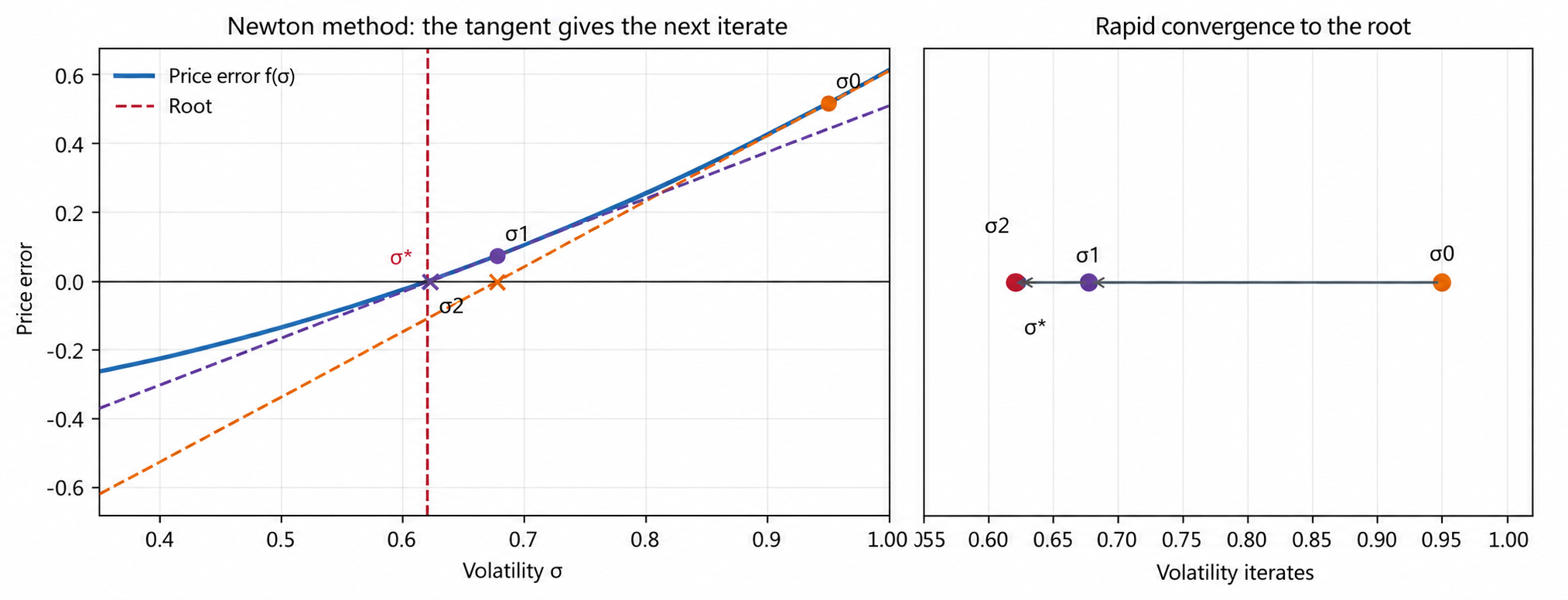
Schematic of the Newton method. The left panel shows the tangent to the price error function at the current iterate. Its intersection with the horizontal axis gives the next volatility estimate. The right panel shows the iterates rapidly approaching the root.
From Formulas to Code
volatility and next_volatility correspond to \(\sigma_m\) and \(\sigma_{m+1}\). error corresponds to \(f(\sigma_m)\), and vega corresponds to \(f\prime(\sigma_m)=\partial V_{\rm BS}/\partial\sigma\); the update is the ratio of the two.
Function 1.13: Implied volatility by Newton iteration
def implied_volatility_newton(
    target, S0, K, T, r, cp, initial=0.20, tolerance=1e-10, max_iterations=20
):
    '''Recover volatility by Newton iteration and return its trace.'''
    if initial <= 0:
        raise ValueError("Initial volatility must be positive")
    volatility = initial
    iteration_rows = []
    for iteration in range(max_iterations):
        price = black_scholes_formula(volatility, S0, K, T, r, cp)
        d1 = (np.log(S0 / K) + (r + volatility**2 / 2) * T) / (
            volatility * np.sqrt(T)
        )
        vega = S0 * norm.pdf(d1) * np.sqrt(T)
        error = price - target
        iteration_rows.append(
            {"Iteration": iteration, "Volatility": volatility, "Price error": error}
        )
        if abs(error) < tolerance:
            break
        if not np.isfinite(vega) or vega <= 0:
            raise ValueError("Invalid Vega for Newton iteration")
        next_volatility = volatility - error / vega
        if not np.isfinite(next_volatility) or next_volatility <= 0:
            raise ValueError("Newton step produced nonpositive volatility")
        volatility = next_volatility
    else:
        raise RuntimeError("Newton iteration did not converge within the specified iteration limit")
    return volatility, pd.DataFrame(iteration_rows)
# Function 1.13 example: Solve for implied volatility and display Newton iterations
newton_volatility, newton_iterations = implied_volatility_newton(
target_price,
iv_spot,
iv_strike,
iv_maturity,
iv_rate,
iv_cp,
)
newton_iterations| Iteration | Volatility | Price error | |
|---|---|---|---|
| 0 | 0 | 0.200000 | 1.247477e+00 |
| 1 | 1 | 0.163389 | 5.811603e-02 |
| 2 | 2 | 0.161490 | 2.212975e-04 |
| 3 | 3 | 0.161483 | 3.319599e-09 |
| 4 | 4 | 0.161483 | 2.131628e-14 |
Newton result. Starting from the initial value \(\sigma_0=0.20\), Newton’s method gives
\[ \sigma_{\mathrm{imp}}^{\mathrm{(Newton)}}\approx 0.161483, \]
that is, an implied volatility of approximately \(16.15\%\). The price error in the last iteration is approximately \(2.1\times10^{-14}\), consistent with the result obtained by bisection.
1.10.3 Implied Volatility Surface
The BSM model uses a fixed volatility, while the implied volatility \(\sigma_{\mathrm{imp}}(K,T)\) inferred from market option prices varies with strike price \(K\) and maturity \(T\). Expressing implied volatility as a function of strike price and maturity defines the volatility surface. Figure 1.17 shows Euro Stoxx 50 implied volatility on January 3, 2018, for strike prices from 2,000 to 5,000 and maturities from two weeks to ten years. The two horizontal axes represent strike price and time to maturity, and the vertical axis represents implied volatility.
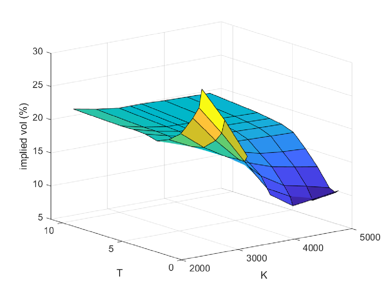
Figure 1.17 Euro Stoxx 50 implied volatility surface on January 3, 2018: strike prices from 2,000 to 5,000 and maturities from two weeks to ten years.
1.10.4 Volatility Skew
We select the options with a maturity of 2 years from the surface above and plot their implied volatilities against strike price in Figure 1.18. The higher the strike price, the lower the implied volatility; this is called volatility skew. Volatility skew emerged after the 1987 stock market crash. One explanation is that equity investors concerned about a crash buy out-of-the-money puts to hedge stock market risk, pushing up the prices and implied volatilities of low-strike puts. Another explanation is that buying in-the-money calls amounts to buying stocks with leverage, increasing demand for these options and raising the prices and implied volatilities of low-strike calls. Bollen and Whaley (2004) found that changes in the implied volatility of S&P 500 index options are related to net buying pressure for put options.
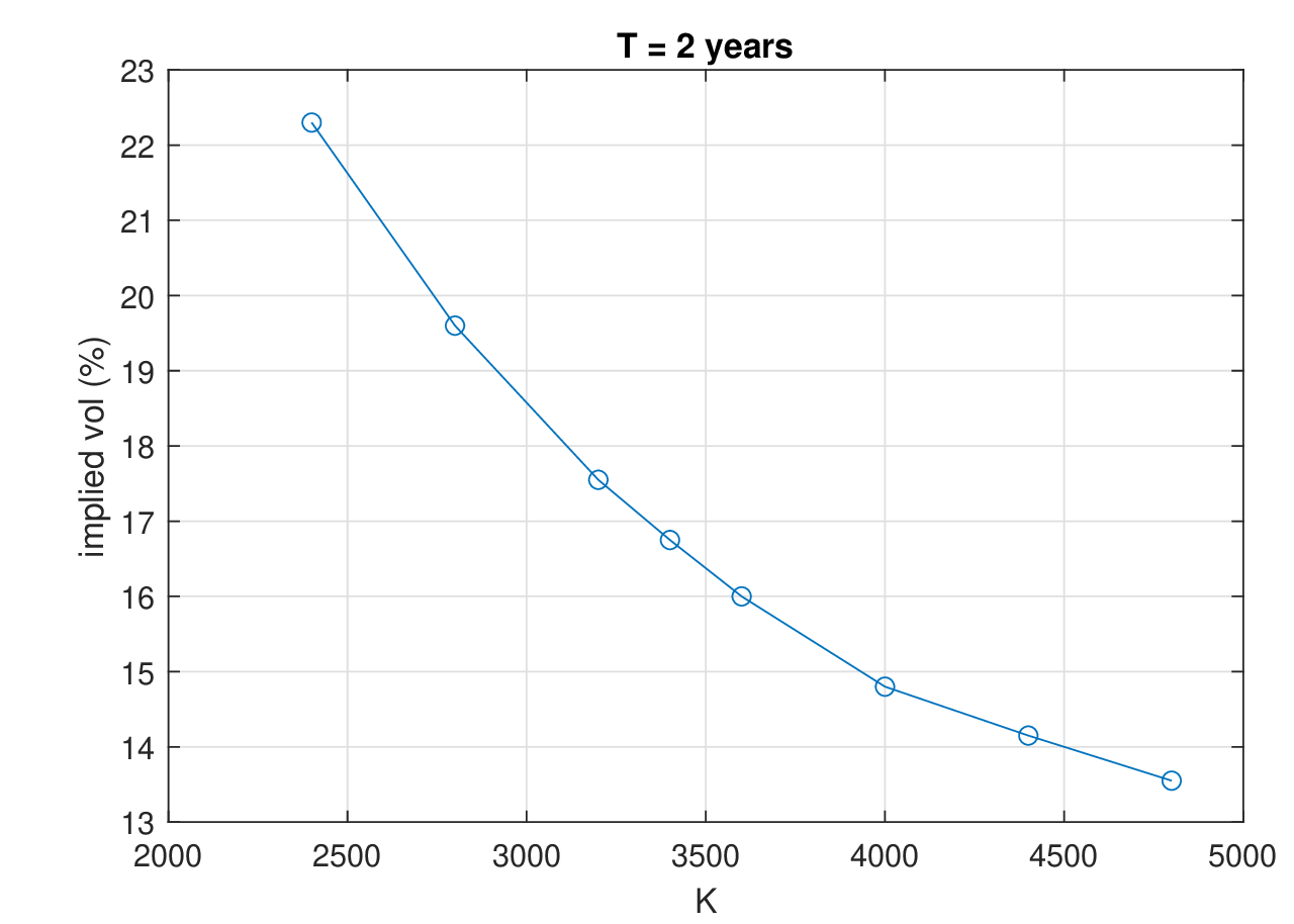
Figure 1.18 Implied volatility versus strike price for two-year Euro Stoxx 50 options on January 3, 2018.
References
Bachelier, L. (1900). “Théorie de la spéculation.” Annales scientifiques de l’École Normale Supérieure, Series 3, 17, 21–86. https://doi.org/10.24033/asens.476
Samuelson, P. A. (1965). “Rational Theory of Warrant Pricing.” Industrial Management Review, 6(2), 13–32.
Merton, R. C. (1976). “Option Pricing When Underlying Stock Returns Are Discontinuous.” Journal of Financial Economics, 3, 125–144.
Kou, S. G. (2002). “A Jump Diffusion Model for Option Pricing.” Management Science, 48, 1086–1101.
Beckers, S. (1981). “A Note on Estimating the Parameters of the Diffusion-Jump Model of Stock Returns.” Journal of Financial and Quantitative Analysis, 16(1), 127–140.
Madan, D., Carr, P., & Chang, E. (1998). “The Variance Gamma Process and Option Pricing.” European Finance Review, 2, 79–105.
Figueroa-López, J. E., Lancette, S. R., Lee, K., & Mi, Y. (2011). “Estimation of NIG and VG Models for High Frequency Financial Data.” In Handbook of Modeling High-Frequency Data in Finance, 1–25. John Wiley & Sons.
Barndorff-Nielsen, O. E. (1997). “Normal Inverse Gaussian Distributions and Stochastic Volatility Modelling.” Scandinavian Journal of Statistics, 24, 1–13.
Schoutens, W. (2003). Lévy Processes in Finance: Pricing Financial Derivatives. John Wiley & Sons.
Cox, J., & Ross, S. (1976). “The Valuation of Options for Alternative Stochastic Processes.” Journal of Financial Economics, 3, 145–166.
Black, F., & Scholes, M. (1973). “The Pricing of Options and Corporate Liabilities.” Journal of Political Economy, 81, 637–654.
Aït-Sahalia, Y. (2004). “Disentangling Diffusion from Jumps.” Journal of Financial Economics, 74, 487–528.
Bollen, N. P. B., & Whaley, R. E. (2004). “Does Net Buying Pressure Affect the Shape of Implied Volatility Functions?” The Journal of Finance, 59(2), 711–753. https://doi.org/10.1111/j.1540-6261.2004.00647.x