1.1 期权简介

随机过程与风险中性定价

本章从期权收益出发，介绍布朗运动、几何布朗运动及 Merton跳跃扩散、Variance Gamma、Normal Inverse Gaussian 等进阶模型，再通过风险中性定价引出 Black–Scholes 公式、敏感性参数和隐含波动率。重点是理解模型如何描述价格变化，以及如何从模型参数计算期权价格、从市场期权价格求解隐含波动率。

# 导入本节所需的计算、统计和绘图库
import sys
from pathlib import Path

import matplotlib.pyplot as plt
import numpy as np
import pandas as pd
import yfinance as yf
from scipy.integrate import quad
from scipy.stats import kurtosis, norm, poisson, skew

project_root = Path.cwd()
while not (project_root / "src").exists() and project_root != project_root.parent:
    project_root = project_root.parent
sys.path.insert(0, str(project_root / "src"))

plt.style.use("seaborn-v0_8-whitegrid")
plt.rcParams["font.family"] = "sans-serif"
plt.rcParams["font.sans-serif"] = [
    "Microsoft YaHei", "PingFang SC", "Noto Sans CJK SC",
    "WenQuanYi Micro Hei", "SimHei", "DejaVu Sans",
]
plt.rcParams["axes.unicode_minus"] = False
np.set_printoptions(precision=6, suppress=True)
pd.set_option("display.precision", 6)

期权是一种金融衍生证券，其价值衍生于标的资产；标的资产可以是商品、股票、外汇、利率或指数。买方先支付权利金，获得按约定条件交易的权利但没有义务；卖方收取权利金，并在买方行权时承担履约义务。

我们先区分三种分类方式： 看涨或看跌描述收益方向；欧式、美式或百慕大描述可以行权的时间；亚式、价差和篮子期权描述收益依赖哪些价格信息。

看涨期权与看跌期权

看涨期权（call，也称认购期权或买入期权）赋予买方按行权价买入标的资产的权利，通常用于表达对价格上涨的看法，或锁定未来的买入价格。例如，若行权价 \(K=100\)，到期时标的价格 \(S_T=120\)，买方可以按 100 买入价值 120 的资产，因此获得 20 的到期收益；若 \(S_T=80\)，买方不会按 100 行权，收益为 0。欧式看涨期权在到期日 \(T\) 的收益为

\[g_C(S_T) = \max(S_T-K,0) = (S_T-K)^+\tag{1.1.1}.\]

看跌期权（put，也称认沽期权或卖出期权）赋予买方按行权价卖出标的资产的权利，通常用于表达对价格下跌的看法，或为已有持仓提供类似保险的保护。例如，若 \(K=100\) 且 \(S_T=80\)，买方可以按 100 卖出价值 80 的资产，获得 20 的到期收益；若 \(S_T=120\)，按 100 卖出没有好处，收益为 0。欧式看跌期权的收益为

\[g_P(S_T) = \max(K-S_T,0) = (K-S_T)^+\tag{1.1.2}.\]

式（1.1.1）和式（1.1.2）给出的是到期收益，其中 \(S_T\) 是到期日的标的资产价格，\(K\) 是行权价，不含买方先支付的权利金；若忽略权利金的资金时间价值，买方的到期净损益是收益减去权利金 \(p\)；若把时刻 0 支付的权利金按无风险利率 \(r\) 换算到到期日，则净损益为 \(g(S_T)-pe^{rT}\)。卖方在相同计息约定下的净损益则相反。

欧式看涨期权（左）和看跌期权（右）在到期日的收益函数。

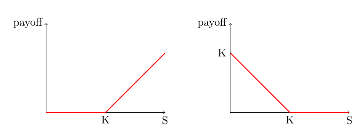
图 1.1 欧式看涨期权（左）和看跌期权（右）在到期日的收益函数。

行权时间：欧式、美式和百慕大

欧式期权只能在到期日行权；美式期权（American option）和百慕大期权（Bermudan Option）则可以在更多时刻行权。三者都可以是看涨或看跌，差别在于买方什么时候可以行权：欧式只能在期权到期日 \(T\) 行权，美式可以在期权到期前任意时间行权，百慕大介于两者之间，可以在预先规定的时点 \(0<T_1<T_2<\cdots<T_M\leq T\) 行权。提前行权的机会会改变期权价值，因此美式和百慕大期权不能只看期权到期日资产价格 \(S_T\)，还要考虑价格路径和每个可能行权时点。

收益依赖价格路径

亚式期权（Asian option）的收益取决于一段期间内的资产平均价格，而不是某一个时点的价格。若 \(A(T)\) 是区间 \([0,T]\) 内的连续或离散平均价格，亚式看涨期权的收益为 \([A(T)-K]^+\)，对应的看跌期权可写为 \([K-A(T)]^+\)。例如 \(K=100\)、平均价格 \(A(T)=105\) 时，看涨期权收益为 5，即使到期日当天的价格低于 100 也不改变这个结果。平均价格会平滑短期波动，因此这类期权对到期日附近的单日价格冲击不那么敏感，也常用于降低结算时点价格被操纵的影响。

亚式看涨期权示意图：平均价格决定到期收益。

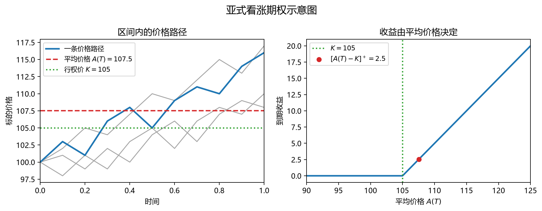
图 1.1a 亚式看涨期权示意图：收益由区间平均价格 \(A(T)\) 决定。

收益基于多个标的资产

价差期权（spread option）同时看两个标的的相对表现。例如，价差看涨期权可以写成 \([S_T^{(1)}-S_T^{(2)}-K]^+\)：若 \(S_T^{(1)}=110\)、\(S_T^{(2)}=100\)、\(K=5\)，收益为 5；只有资产 1 的价格相对资产 2 高出行权价 \(K\) 时才产生收益。

篮子期权（basket option）则把多个标的合成为一个篮子，若 \(B_T=\sum_{i=1}^n w_iS_T^{(i)}\)，篮子看涨期权的收益为 \([B_T-K]^+\)；例如权重为 0.6 和 0.4、两个标的价格分别为 120 和 80 时，篮子价格为 104，若 \(K=100\) 则收益为 4。权重 \(w_i\) 决定每个标的对收益的贡献。

价差看涨期权示意图：两个标的的价格之差决定到期收益。

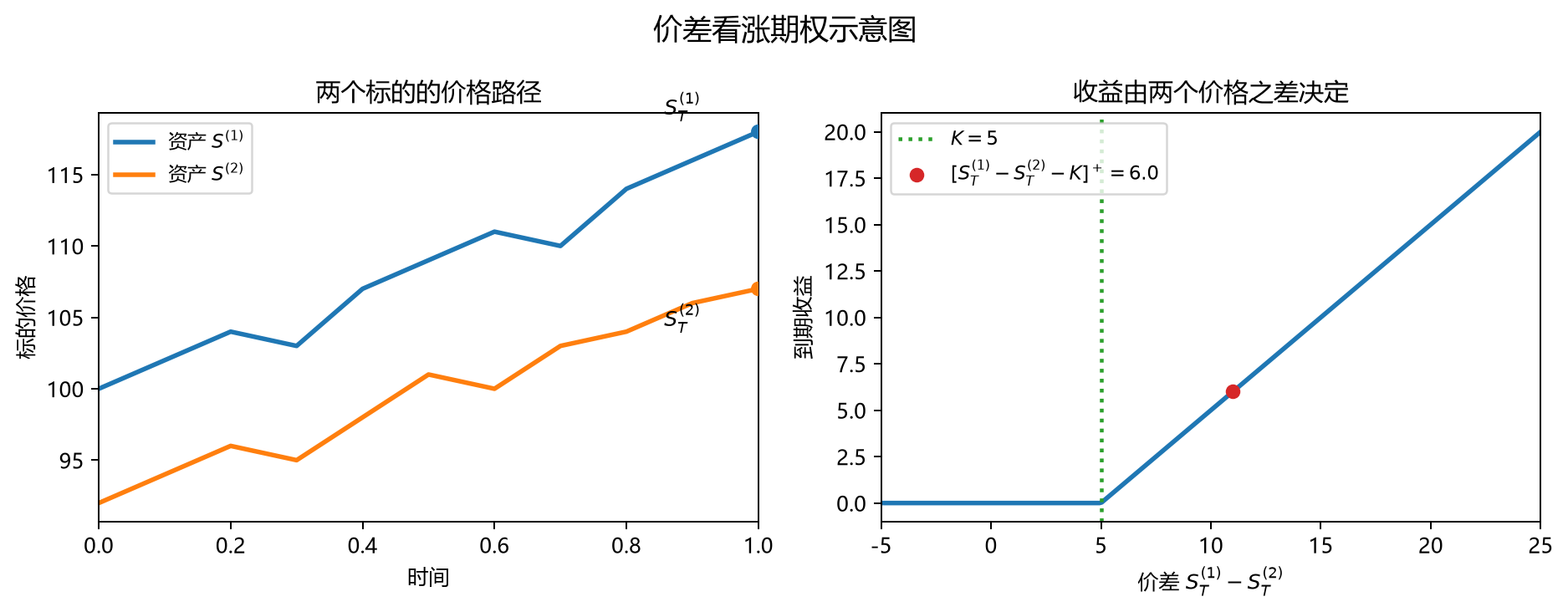
图 1.1b 价差看涨期权示意图：收益由两个标的价格之差 \(S_T^{(1)}-S_T^{(2)}\) 决定。

本章先用欧式看涨和看跌期权建立定价的基本理论和方法，以后章节会涉及如何处理美式期权，路径依赖和多标期权。

1.2 资产价格随机过程

记当前时刻为 \(t=0\)。考虑标的资产为股票的期权。决定欧式期权价格最重要的因素是标的股票在期权到期日 \(t=T\) 的价格 \(S_T\)。而对于美式和亚式期权，则期权价格与标的资产在期权到期日 \(T\) 之前的价格 \(S_t,0 \leq t\leq T\) 都相关。

因为股票在将来的价格 \(S_t,t>0\) 在 \(t=0\) 时不可知，所以对于任意给定时间 \(t>0\) 的资产价格 \(S_t\) 可以看作是一个随机变量（random variable），而在时间段 \((0,T]\) 内的资产价格 \(S_t,0<t\leq T\) 可以看作是一个随机过程（stochastic process）。所以对期权进行定价的一个很重要的问题是：用什么随机过程来描述股票价格？

早在20世纪初，Bachelier（1900）提出用布朗运动（Brownian Motion，详见第 1.3 节）来描述股票价格。简单来说，对于任意时间 \(t>0\)，股价 \(S_t\) 服从正态分布。由于正态分布定义域为 \((-\infty,+\infty)\)，所以该模型的一个明显缺陷是无法确保股价 \(S_t>0\)。

为了保证股价为正，Samuelson（1965）提出用布朗运动来描述股价的对数收益，

\[X_t=\log S_t-\log S_0\tag{1.2.1}\]

而非股价本身。此时股票价格 \(\{S_t=S_0\exp(X_t);0<t\leq T\}\) 服从几何布朗运动（Geometric Brownian Motion）。至于为什么选择对数收益而不是普通收益的原因在于

1. 首先对数收益率与普通收益率（\(X_t'=S_t/S_0-1\)）在价格变动很小的情况下近似相等，这可以由指数函数的泰勒级数（Taylor series）\(e^X \approx 1+X\) 推出。
2. 其次，指数形式 \(S_t=S_0e^{X_t}\) 使股票价格始终为正；
3. 最后对数收益可以简单相加得到累计收益。我们举一个最简单的例子。假如 \(S_1=S_0e^{X_1}\)，\(S_2=S_1e^{X_2}\)，\(S_3=S_2e^{X_3}\)，那么 \(S_3\) 也可表示为 \(S_3=S_0e^{X_1+X_2+X_3}\)。并且当 \(X_1,X_2,X_3\) 独立并均服从正态分布时，\(X_1+X_2+X_3\) 同样服从正态分布。如果使用普通收益率，当 \(S_1=S_0(1+X_1')\)，\(S_2=S_1(1+X_2')\) 和 \(S_3=S_2(1+X_3')\) 时，可以得到 \(S_3=S_0(1+X_1')(1+X_2')(1+X_3')=S_0(1+X_1'+X_2'+X_3'+X_1'X_2'+X_2'X_3'+X_1'X_3'+X_1'X_2'X_3')\)，这比使用对数收益率要复杂得多。问题更大的是，当 \(X_1',X_2',X_3'\) 独立且都服从正态分布，\(X_1'X_2'\) 等项并不服从正态分布，所以 \(S_2,S_3\) 的概率分布会很复杂。

接下去我们将主要介绍四种可用于描述 \(X_t\) 的随机过程：布朗运动，跳跃扩散（Jump Diffusion），Variance Gamma 过程以及 Normal Inverse Gaussian 过程。

1.3 布朗运动

记 \(N(\mu,\sigma^2)\) 为均值为 \(\mu\)、方差为 \(\sigma^2\) 的正态分布（normal distribution，也称 Gaussian distribution）。令随机变量 \(X\) 服从正态分布 \(N(\mu,\sigma^2)\)，则 \(X\) 的概率密度函数为

\[f(x;\mu,\sigma)=\frac{1}{\sqrt{2\pi}\sigma} \exp\left(-\frac{(x-\mu)^2}{2\sigma^2}\right).\]

当 \(\mu=0\) 且 \(\sigma=1\) 时，称 \(X\) 服从标准正态分布，并记其密度为 \(\phi(x)\)，分布函数为 \(\Phi(x)\)。图 1.2 给出了不同参数的正态分布概率密度函数。不难看出：

• 正态分布的概率密度函数曲线呈钟形，这类曲线被称为钟形曲线（bell curve）；
• 正态分布在位置参数 \(\mu\) 两端对称，\(\mu\) 决定了分布的中心，\(\mu\) 越大，分布位置越往右；
• \(\sigma\) 决定了分布的离散度（dispersion），\(\sigma\) 越大，分布越为分散，尾部越长。

# 图 1.2：不同均值和方差对应的正态分布概率密度函数
normal_grid = np.linspace(-6.0, 6.0, 500)
fig, ax = plt.subplots(figsize=(7, 4))
ax.plot(normal_grid, norm.pdf(normal_grid), color="red",
        label=r"$\mu=0,\sigma^2=1$")
ax.plot(normal_grid, norm.pdf(normal_grid, loc=1.0),
        color="blue", linestyle="--", label=r"$\mu=1,\sigma^2=1$")
ax.plot(normal_grid, norm.pdf(normal_grid, scale=np.sqrt(2)),
        color="black", linestyle="-.", label=r"$\mu=0,\sigma^2=2$")
ax.set_xlim(-6, 6)
ax.set_ylim(0, 0.4)
ax.set_xticks(np.arange(-6, 7, 2))
ax.set_yticks(np.arange(0, 0.401, 0.05))
ax.tick_params(direction="in", top=True, right=True)
ax.legend(loc="upper right", frameon=True, fancybox=False,
          facecolor="white", edgecolor="black")
fig.tight_layout()
plt.show()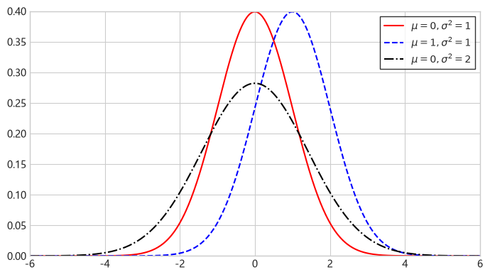

图 1.2 对应不同参数的正态分布概率密度函数。

标准布朗运动（standard Brownian motion，也称为 Wiener 过程）满足以下条件：

1. \(W_0=0\)；
2. \(W\) 的增量相互独立，即对于任意时间 \(t_1<t_2\leq t_3<t_4\)，\(W_{t_4}-W_{t_3}\) 与 \(W_{t_2}-W_{t_1}\) 相互独立；
3. \(W\) 的增量服从正态分布，对于所有 \(t_2>t_1\)，\(W_{t_2}-W_{t_1}\sim\mathcal{N}(0,t_2-t_1)\)；
4. \(W\) 的路径连续，不存在跳跃。

令 \(X_t=\mu t+\sigma W_t\)，其中 \(\mu\) 和 \(\sigma\) 均为常数，则 \(X_t\) 被称为带漂移的布朗运动。不难得出，\(X_t\) 在任意时间 \(h>0\) 的增量 \(X_h=X_{t+h}-X_t\) 的边际分布是正态分布 \(X_h\sim\mathcal{N}(\mu h,\sigma^2h)\)。所以 \(\mu\) 表示单位时间的漂移，被称为漂移率，而 \(\sigma\) 表示单位时间内 \(X\) 的标准差，称为波动率。增量均值按 \(h\) 增长，标准差按 \(\sqrt h\) 增长：时间从 1 年增加到 4 年，均值扩大到 4 倍，标准差扩大到 2 倍。

图 1.3 给出了 \(\mu=0.1,\sigma=0.3\) 时 \(X_t\) 的五条样本路径（sample path）。

# 带漂移布朗运动的样本路径
brownian_rng = np.random.default_rng(42)
brownian_steps = 500
brownian_paths_count = 5
brownian_time = np.linspace(0.0, 1.0, brownian_steps + 1)
brownian_dt = brownian_time[1] - brownian_time[0]
brownian_drift = 0.10
brownian_volatility = 0.30
brownian_increments = (
    brownian_drift * brownian_dt
    + brownian_volatility
    * np.sqrt(brownian_dt)
    * brownian_rng.standard_normal(
        (brownian_paths_count, brownian_steps)
    )
)
drifted_brownian_paths = np.column_stack(
    [np.zeros(brownian_paths_count), np.cumsum(brownian_increments, axis=1)]
)

# 图 1.3：带漂移布朗运动的样本路径
fig, ax = plt.subplots(figsize=(8, 4.2))
ax.plot(brownian_time, drifted_brownian_paths.T, alpha=0.25)
ax.set_xlabel("时间")
ax.set_ylabel("$X_t$")
ax.set_title("带漂移布朗运动的样本路径")
ax.grid(True, alpha=0.25)
fig.tight_layout()
plt.show()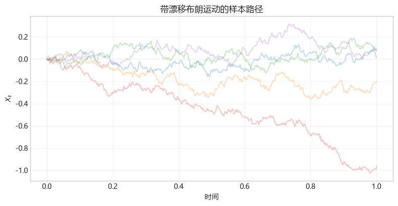

图 1.3 带漂移的布朗运动的样本路径。

图 1.4 中，蓝色实线展示了 \(X_t\) 在 \(t=1,3,5\) 时的边际分布 \(X_t\sim\mathcal{N}(\mu t,\sigma^2t)\)，黑色实线和红色虚线则分别给出了根据 \(X_t\) 的边际分布推出的在 \(t\in[0,6]\) 时的均值和逐时点约 95% 的分布范围。其中 95% 分布范围由 \(\mu t\pm1.96\sigma\sqrt t\)给出。显然，随着时间\(t\)增长，\(X_t\) 的分布越为发散。

# 图 1.4：带漂移布朗运动在不同时刻的边际分布
brownian_marginal_times = np.array([1.0, 3.0, 5.0])
marginal_grid = np.linspace(-1.5, 2.2, 500)
marginal_densities = [
    norm.pdf(
        marginal_grid,
        loc=brownian_drift * time_value,
        scale=brownian_volatility * np.sqrt(time_value),
    )
    for time_value in brownian_marginal_times
]
marginal_mean = brownian_drift * brownian_time
marginal_lower = marginal_mean - 1.96 * brownian_volatility * np.sqrt(
    brownian_time
)
marginal_upper = marginal_mean + 1.96 * brownian_volatility * np.sqrt(
    brownian_time
)
marginal_path_rng = np.random.default_rng(43)
marginal_path_time = np.linspace(0.0, 6.0, 601)
marginal_path_dt = marginal_path_time[1] - marginal_path_time[0]
marginal_path_count = 20
marginal_path_increments = (
    brownian_drift * marginal_path_dt
    + brownian_volatility
    * np.sqrt(marginal_path_dt)
    * marginal_path_rng.standard_normal((marginal_path_count, 600))
)
marginal_paths = np.column_stack(
    [
        np.zeros(marginal_path_count),
        np.cumsum(marginal_path_increments, axis=1),
    ]
)
marginal_path_mean = brownian_drift * marginal_path_time
marginal_path_lower = marginal_path_mean - 1.96 * brownian_volatility * np.sqrt(
    marginal_path_time
)
marginal_path_upper = marginal_path_mean + 1.96 * brownian_volatility * np.sqrt(
    marginal_path_time
)

fig = plt.figure(figsize=(8, 5.5))
ax = fig.add_subplot(111, projection="3d")
for time_value, density in zip(brownian_marginal_times, marginal_densities):
    ax.plot(
        np.full_like(marginal_grid, time_value),
        marginal_grid,
        density,
        color="tab:blue",
    )
ax.plot(
    marginal_path_time,
    marginal_path_mean,
    np.zeros_like(marginal_path_time),
    color="black",
)
ax.plot(
    marginal_path_time,
    marginal_path_lower,
    np.zeros_like(marginal_path_time),
    color="red",
    linestyle="--",
)
ax.plot(
    marginal_path_time,
    marginal_path_upper,
    np.zeros_like(marginal_path_time),
    color="red",
    linestyle="--",
)
for path in marginal_paths:
    ax.plot(
        marginal_path_time,
        path,
        np.zeros_like(marginal_path_time),
        color="limegreen",
        linestyle="--",
        alpha=0.35,
    )
ax.set_xlabel("$t$")
ax.set_ylabel("$X_t$")
ax.set_zlabel("pdf")
ax.set_title("带漂移布朗运动在不同时刻的边际分布")
fig.tight_layout()
plt.show()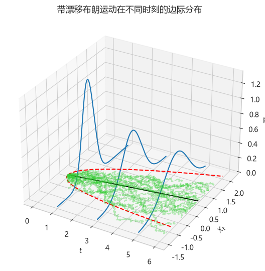

图 1.4 带漂移的布朗运动在不同时刻的边际分布。

正态增量的均值及二至四阶中心矩如下。本章用 \(\mu_1\) 表示均值，用 \(\mu_k\)（\(k\geq2\)）表示中心矩。一阶中心矩为 \(E[X_h-E[X_h]]=0\)。

\[ \begin{aligned} \mu_1 &= E [X_h] = \mu h,\\ \mu_2 &= E [(X_h - E[X_h])^2] = \sigma^2 h,\\ \mu_3 &= E [(X_h - E[X_h])^3] = 0,\\ \mu_4 &= E [(X_h - E[X_h])^4] = 3\sigma^4 h^2. \end{aligned} \]

其中一阶矩就是均值，二阶中心矩是方差。将三阶矩和四阶矩标准化，可以得到描述分布函数的另外两个重要特征值：偏度（skewness）和峰度（kurtosis）。它们定义如下

\[ \begin{aligned} Skw &:= \frac{\mu_3}{\mu_2^{3/2}}, \quad Krt := \frac{\mu_4}{\mu_2^2}. \end{aligned} \]

显然正态分布的偏度为 0、峰度为 3。此外，将峰度减去 3 可以得到超额峰度（excess kurtosis），正态分布的超额峰度为 0。在此我们指出，在相应矩存在的条件下，对称分布的偏度为 0，峰度大于 3（超额峰度大于 0）的分布称为尖峰态（leptokurtic）。峰度把标准化偏离幅度提升到四次方后取平均，因此对极端值特别敏感：偏离均值 4 个标准差的观测贡献为 \(4^4=256\)，偏离 2 个标准差的贡献为 \(2^4=16\)，前者是后者的 16 倍。

当 \(X_t=\mu t+\sigma W_t\) 用于描述股票对数收益时，股票价格

\[\frac{S_t}{S_0}=e^{X_t}=e^{\mu t+\sigma W_t}\]

服从几何布朗运动（geometric Brownian motion）。对于任意给定 \(t\)，\(S_t/S_0\) 的边际分布是对数正态分布（lognormal distribution）：

\[\frac{S_t}{S_0}\sim\operatorname{Lognormal}(\mu t,\sigma^2t).\]

根据对数正态分布的性质，\(S_t/S_0\) 的期望和方差分别为

\[E\left[\frac{S_t}{S_0}\right]=\frac{E[S_t]}{S_0}=e^{(\mu+\sigma^2/2)t},\]

\[\begin{aligned} \operatorname{Var}\left[\frac{S_t}{S_0}\right] &=E\left[\left(\frac{S_t}{S_0}\right)^2\right]-E\left[\frac{S_t}{S_0}\right]^2 \\ &=e^{2(\mu+\sigma^2)t}-e^{(2\mu+\sigma^2)t} \\ &=e^{(2\mu+\sigma^2)t}(e^{\sigma^2t}-1). \end{aligned}\]

这一模型最早由 Samuelson（1965）提出，因此也被称为 Samuelson 模型。

这里 \(\mu\) 是对数收益 \(X_t\) 的漂移率，\(E[X_t]=\mu t\)。股票的期望价格则按 \(\mu+\sigma^2/2\) 增长，因为正态随机项满足 \(E[e^{\sigma W_t}]=e^{\sigma^2t/2}\)，从而 \(E[S_t]/S_0=e^{(\mu+\sigma^2/2)t}\)。

1.3.1 几何布朗运动拟合 S&P 500 指数

接下来我们演示如何通过矩估计（Method of Moments）来用几何布朗运动拟合 2000 年 1 月 1 日至 2013 年 6 月 28 日的 S&P 500 指数。

S&P 500 指数的历史数据可以通过 Yahoo Finance 获取。以下程序可下载 ^GSPC 在 2000 年 1 月至 2013 年 6 月 28 日的历史数据；下载结果保存在当前会话的内存中，供本章后续计算使用。Yahoo Finance 的结束日期不包含在下载区间内，因此程序将 end 设为 2013-06-29。程序设置 auto_adjust=False，选取 Adj Close 字段，并将该列重命名为 close，以便后续公式使用统一的价格变量。对于个股，Adjusted Close 包含拆股和分红调整。

# 下载 S&P 500 历史数据
sp500_data = yf.download(
    "^GSPC", start="2000-01-01", end="2013-06-29",
    auto_adjust=False, multi_level_index=False, progress=False,
)
sp500_data = sp500_data.rename_axis("date").reset_index()
sp500_data["close"] = pd.to_numeric(sp500_data["Adj Close"])
sp500_data = (
    sp500_data[["date", "close"]]
    .sort_values("date")
    .dropna(subset=["close"])
    .reset_index(drop=True)
)
print("数据来源：Yahoo Finance: ^GSPC Adj Close（本次下载）")
print(f"观测数：{len(sp500_data):,}；区间："
      f"{sp500_data['date'].iloc[0]:%Y-%m-%d} 至 "
      f"{sp500_data['date'].iloc[-1]:%Y-%m-%d}")
sp500_data.head()

# 图 1.5：2000 年 1 月至 2013 年 6 月 S&P 500 的调整收盘价序列
fig, ax = plt.subplots(figsize=(10, 4.2))
ax.plot(sp500_data["date"], sp500_data["close"])
ax.set_xlabel("日期")
ax.set_ylabel("指数水平")
ax.set_title("S&P 500 调整收盘价")
plt.show()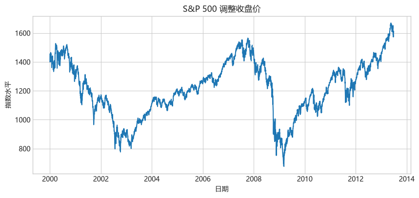

图 1.5 2000 年 1 月至 2013 年 6 月 S&P 500 的调整收盘价序列。

Yahoo Finance 中常用的股票指数代码如下。下载其他指数时，只需把 yf.download 的代码替换为表中的相应值。

Yahoo Finance 代码	股票指数
^GSPC	S&P 500
^DJI	Dow Jones Industrial Average
^IXIC	Nasdaq Composite
^FTSE	FTSE 100
^GDAXI	DAX
^FCHI	CAC 40
^STOXX50E	Euro Stoxx 50
^HSI	Hang Seng Index
000001.SS	Shanghai Composite
^N225	Nikkei 225

表 1.1 Yahoo Finance 中常用的股票指数代码。

我们将对每日调整收盘指数进行分析。首先计算每日对数收益。图 1.6 显示了 2000 年 1 月至 2013 年 6 月 S&P 500 指数的对数收益。

\[ x_i=\log(S_i)-\log(S_{i-1}),\quad i=1,\ldots,n \tag{1.3.1} \]

# 计算日对数收益
log_returns = np.diff(np.log(sp500_data["close"].to_numpy()))
return_dates = sp500_data["date"].iloc[1:]

# 图 1.6：2000 年 1 月至 2013 年 6 月的 S&P 500 日对数收益率
fig, ax = plt.subplots(figsize=(10, 4.2))
ax.plot(return_dates, log_returns)
ax.set_xlabel("日期")
ax.set_ylabel("对数收益")
ax.set_title("S&P 500 日对数收益")
plt.show()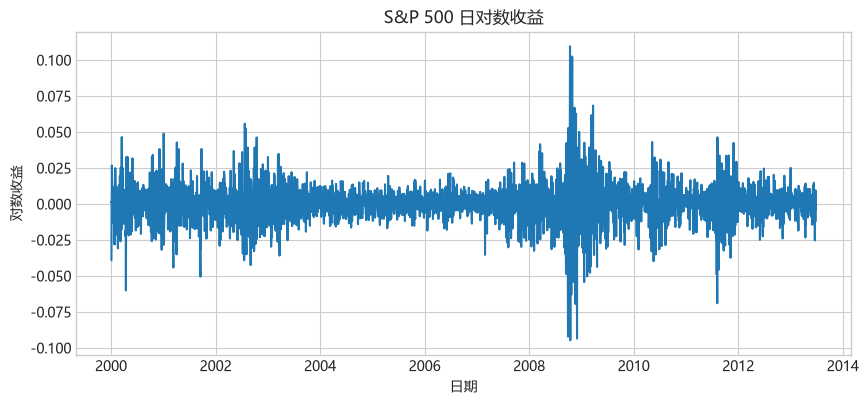

图 1.6 2000 年 1 月至 2013 年 6 月的 S&P 500 日对数收益率。

本章的矩估计统一使用经验中心矩：二阶及以上中心矩均以 \(n\) 为分母，偏度和峰度也直接由这些中心矩计算，不额外作有限样本偏差修正。接下来计算对数收益的样本均值和方差，

\[ \widehat\mu_{1,n}=\frac{1}{n}\sum_{i=1}^n x_i,\quad \widehat{\operatorname{Var}}_n=\frac{1}{n} \sum_{i=1}^n(x_i-\widehat\mu_{1,n})^2.\]

然后计算样本频率 \(h=T/n\)，其中 \(T\) 代表样本时长。GBM 假设每日对数收益服从 \(\mathcal{N}(\mu h,\sigma^2h)\)，因此样本均值和样本方差给出

\[ \widehat\mu=\frac{\widehat\mu_{1,n}}{h},\quad \widehat\sigma=\sqrt{\frac{\widehat{\operatorname{Var}}_n}{h}}.\]

这里用观测区间的日历长度除以收益增量个数定义 \(h\)，因此 \(h\) 是以年为单位的平均观测间隔，约为 \(1/252\)。年化时，日对数收益的均值按时间间隔 \(h\) 换算，标准差则按 \(\sqrt h\) 换算，因为方差与时间长度成正比。例如取 \(h=1/252\)，若日收益标准差为 \(1\%\)，对应的年化波动率约为 \(1\%\times\sqrt{252}=15.9\%\)。以上步骤可由下面程序实现。

# 计算GBM 矩估计和样本统计量
sample_years = (
    sp500_data["date"].iloc[-1] - sp500_data["date"].iloc[0]
).days / 365.25
time_step = sample_years / len(log_returns)
sample_mean = np.mean(log_returns)
sample_variance = np.var(log_returns, ddof=0)
drift = sample_mean / time_step
volatility = np.sqrt(sample_variance / time_step)
sample_skewness = skew(log_returns, bias=True)
sample_kurtosis = kurtosis(log_returns, fisher=False, bias=True)
sample_excess_kurtosis = sample_kurtosis - 3.0
pd.Series(
    {
        "时间步长": time_step,
        "漂移率": drift,
        "波动率": volatility,
        "偏度": sample_skewness,
        "峰度": sample_kurtosis,
    }
)

时间步长     0.003975
漂移率      0.007325
波动率      0.211596
偏度      -0.167776
峰度      10.469578
dtype: float64

矩估计得到的漂移率和波动率见上方程序输出。此外样本峰度约为 10.5，远远超出正态分布的峰度 3，说明 S&P 500 指数的对数收益呈现厚尾。图 1.7 显示将每日对数收益拟合为正态分布的效果。很明显，S&P 500 指数的对数收益呈现尖峰厚尾，正态分布严重低估了极端收益发生的概率。

综上所述：正态分布并不足以准确地刻画 S&P 500 指数每日对数收益分布。因此，在第 1.4 节至第 1.6 节中我们将介绍三种拟合效果更好的随机过程：跳跃扩散模型、Variance Gamma 模型和 Normal Inverse Gaussian 模型。这三种模型与几何布朗运动最大的不同在于它们都属于带有跳跃的随机过程，而几何布朗运动则是一个连续的随机过程。

# 图 1.7：正态分布对 S&P 500 日对数收益率的整体分布和左尾拟合
normal_lower = -0.10
normal_upper = 0.11
normal_bin_count = 50
normal_bin_width = (normal_upper - normal_lower) / normal_bin_count
fit_bin_edges = np.linspace(normal_lower, normal_upper, normal_bin_count + 1)
fit_bin_centres = (fit_bin_edges[:-1] + fit_bin_edges[1:]) / 2
normal_grid = fit_bin_centres
normal_bin_counts = len(log_returns) * np.diff(
    norm.cdf(fit_bin_edges, loc=sample_mean, scale=np.sqrt(sample_variance))
)
fitted_normal = normal_bin_counts

def model_bin_counts(density, centre=None):
    """Integrate each density over the common bins, splitting at a singularity."""
    return len(log_returns) * np.array([
        quad(density, left, right,
             points=[centre] if centre is not None and left < centre < right else None)[0]
        for left, right in zip(fit_bin_edges[:-1], fit_bin_edges[1:])
    ])

left_tail_cutoff = -0.02
left_tail_lower = -0.10
left_tail_bin_count = normal_bin_count
left_tail_grid = np.linspace(left_tail_lower, left_tail_cutoff, 300)
left_tail_normal = (
    norm.pdf(
        left_tail_grid,
        loc=sample_mean,
        scale=np.sqrt(sample_variance),
    )
    * len(log_returns)
    * normal_bin_width
)
fig, axes = plt.subplots(1, 2, figsize=(11, 4.2))
axes[0].hist(
    log_returns,
    bins=fit_bin_edges,
    range=(normal_lower, normal_upper),
    color="0.75",
    edgecolor="blue",
    linewidth=0.8,
    label="样本收益",
)
axes[0].plot(
    normal_grid,
    fitted_normal,
    color="red",
    linewidth=1.8,
    label="GBM 预期频数",
)
axes[0].set_xlabel("对数收益")
axes[0].set_ylabel("频数")
axes[0].set_title("整体分布")
axes[0].set_xlim(normal_lower, normal_upper)
axes[0].grid(True, alpha=0.25)
axes[0].legend(frameon=False)

axes[1].hist(
    log_returns,
    bins=fit_bin_edges,
    range=(normal_lower, normal_upper),
    color="0.75",
    edgecolor="blue",
    linewidth=0.8,
    label="样本收益",
)
axes[1].plot(
    left_tail_grid,
    left_tail_normal,
    color="red",
    linewidth=1.8,
    label="GBM 预期频数",
)
axes[1].set_xlabel("对数收益")
axes[1].set_ylabel("频数")
axes[1].set_title("左尾")
axes[1].set_xlim(left_tail_lower, left_tail_cutoff)
axes[1].set_xticks(np.arange(-0.10, -0.019, 0.02))
axes[1].set_ylim(0.0, 50.0)
axes[1].grid(True, alpha=0.25)
axes[1].legend(frameon=False)
fig.tight_layout()
plt.show()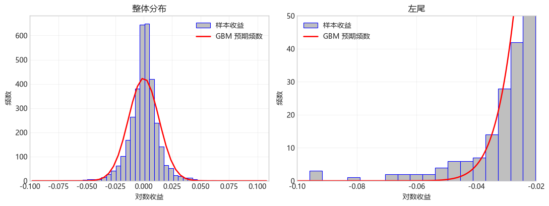

图 1.7 GBM拟合的 2000 年 1 月至 2013 年 6 月 S&P 500 指数的对数收益。

1.4 Merton 跳跃扩散模型

改进 S&P 500 指数每日对数收益历史数据的拟合度的一个可能的解决方案，是在带漂移的布朗运动的基础上加入随机的跳跃

\[X_t=\mu t+\sigma W_t+\sum_{i=1}^{N_t}J_i.\]

其中 \(\sum_{i=1}^{N_t}J_i\) 表示复合泊松（compound Poisson）过程。复合泊松过程有两个随机因素。首先是泊松过程导致资产价格在随机时间产生跳跃，\(N_t\) 表示在 \([0,t]\) 时间段发生跳跃的次数，其概率分布为强度为 \(\lambda t\) 的泊松分布：

\[P(N_t=n)=\frac{e^{-\lambda t}(\lambda t)^n}{n!},\quad n=0,1,\ldots.\]

跳跃强度 \(\lambda\) 衡量跳跃发生的频率。当时间以年计时，\(\lambda\) 的单位为每年。长度为 \(h\) 的区间内，平均跳跃次数为 \(E[N_h]=\lambda h\)，至少发生一次跳跃的概率为 \(1-e^{-\lambda h}\)。对于满足 \(\lambda h\ll1\) 的短区间，该概率近似为 \(\lambda h\)。例如 \(\lambda=12\)、\(h=1/12\) 时，一个月平均发生一次跳跃，但没有跳跃的概率仍为 \(e^{-1}\approx36.8\%\)。

一旦产生跳跃，跳跃幅度 \(J_i\)（\(i=1,\ldots,N_t\)）是独立同分布的随机变量，此外，假设泊松过程、各次跳跃幅度和布朗运动相互独立。Merton（1976）提出跳跃幅度 \(J_i\) 服从正态分布，而 Kou（2002）则使用双指数分布描述跳跃幅度，正向和负向跳跃的条件幅度分别服从指数分布。

本节中我们介绍 Merton（1976）提出的跳跃扩散模型，其中跳跃幅度服从正态分布 \(J_i\sim\mathcal{N}(a,b^2)\)。参数 \(a\) 描述单次对数跳跃的平均跳跃幅度，\(b\) 描述其幅度的离散程度。一次对数跳跃 \(J\) 会使股价乘以 \(e^J\)。保持其他参数不变时，提高 \(\lambda\) 会增加跳跃发生的频率；提高 \(b\) 则使单次跳跃的幅度更不确定。图 1.8 给出了 Merton 跳跃扩散模型的对数收益过程 \(X_t\) 的五条样本路径。

# 图 1.8：设置五条 Merton 对数收益路径的参数
merton_path_rng = np.random.default_rng(17)
merton_path_count = 5
merton_path_step_count = 252
merton_path_time = np.linspace(
    0.0, 1.0, merton_path_step_count + 1
)
merton_path_dt = merton_path_time[1] - merton_path_time[0]
merton_path_drift = 0.08
merton_path_volatility = 0.20
merton_path_jump_intensity = 12.0
merton_path_jump_mean = 0.0
merton_path_jump_std = 0.06

# 图 1.8：生成布朗增量与泊松跳跃并累加路径
merton_path_normals = merton_path_rng.standard_normal(
    (merton_path_count, merton_path_step_count)
)
merton_path_jump_counts = merton_path_rng.poisson(
    merton_path_jump_intensity * merton_path_dt,
    size=(merton_path_count, merton_path_step_count),
)
merton_path_jump_sizes = (
    merton_path_jump_counts * merton_path_jump_mean
    + merton_path_jump_std
    * np.sqrt(merton_path_jump_counts)
    * merton_path_rng.standard_normal(
        (merton_path_count, merton_path_step_count)
    )
)
merton_path_increments = (
    merton_path_drift * merton_path_dt
    + merton_path_volatility * np.sqrt(merton_path_dt) * merton_path_normals
    + merton_path_jump_sizes
)
merton_log_paths = np.column_stack(
    [np.zeros(merton_path_count), np.cumsum(merton_path_increments, axis=1)]
)

# 图 1.8：Merton 跳跃扩散模型对数收益过程的样本路径
fig, ax = plt.subplots(figsize=(8, 4.2))
jump_label_added = False
for path_index, path in enumerate(merton_log_paths):
    (line,) = ax.plot(
        merton_path_time,
        path,
        alpha=0.80,
    )
    jump_steps = np.flatnonzero(merton_path_jump_counts[path_index] > 0) + 1
    if len(jump_steps) > 0:
        ax.scatter(
            merton_path_time[jump_steps],
            path[jump_steps],
            color=line.get_color(),
            s=18,
            zorder=3,
            label="跳跃时点" if not jump_label_added else None,
        )
        jump_label_added = True
ax.set_xlabel("时间")
ax.set_ylabel("对数收益过程 $X_t$")
ax.set_title("Merton 跳跃扩散过程的对数收益样本路径")
ax.grid(True, alpha=0.25)
ax.legend(frameon=False)
plt.show()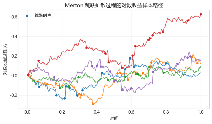

图 1.8 Merton 跳跃扩散模型对数收益过程 \(X_t\) 的五条样本路径。

记 \(X_h=X_{t+h}-X_t\) 为长度为 \(h>0\) 的区间内的增量，\(N_h=N_{t+h}-N_t\) 为 \((t,t+h]\) 内的跳跃次数。如果恰好发生 \(n\) 次跳跃，则增量为

\[ X_h=\underbrace{\mu h}_{\text{漂移项}}+\underbrace{\sigma(W_{t+h}-W_t)}_{\text{扩散项}}+\underbrace{\sum_{i=1}^nJ_i}_{\text{跳跃项之和}}. \]

其中 \(J_i=a+bZ_i\) 为第 \(i\) 次跳跃的幅度，各个 \(Z_i\sim\mathcal{N}(0,1)\) 是相互独立的标准正态随机变量。参数 \(a\) 为单次跳跃幅度的均值，\(b\geq0\) 为其标准差。当 \(n=0\) 时，跳跃项之和为零。

布朗增量满足 \(W_{t+h}-W_t\sim\mathcal{N}(0,h)\)，并且与跳跃次数和跳跃幅度相互独立。给定 \(n\) 次跳跃，跳跃项之和的均值为 \(na\)，方差为 \(nb^2\)。加上独立的扩散项后，增量的条件分布为

\[ X_h\mid N_h=n\sim\mathcal{N}(\mu h+an,\;\sigma^2h+nb^2). \]

从而，\(X_h\) 的无条件概率密度函数为

\[ \begin{aligned} f_{X_h}(x) &=\sum_{n=0}^{\infty} \frac{e^{-\lambda h}(\lambda h)^n}{n!} \frac{1}{\sqrt{2\pi(\sigma^2h+nb^2)}}\\ &\quad\times\exp\left(-\frac{\left[x-(\mu h+na)\right]^2} {2(\sigma^2h+nb^2)}\right). \end{aligned} \]

该概率密度函数是一个无穷级数，可以理解为无穷多个正态分布的混合分布（见 Aït-Sahalia（2004））。计算时可以选择一个足够大的跳跃次数 \(N_{\max}\)作为上限来求和。令 \(\varepsilon\) 为允许省略的 Poisson 右尾概率，并记 \(F^{-1}_{\operatorname{Pois}(\lambda h)}\) 为均值 \(\lambda h\) 的 Poisson 分布分位数，程序取

\[ N_{\max}=F^{-1}_{\operatorname{Pois}(\lambda h)}(1-\varepsilon), \qquad f_{X_h}(x)\approx\sum_{n=0}^{N_{\max}}P(N_h=n)\,f_{X_h\mid N_h=n}(x). \]

也就是说，保留 \(n=0,1,\ldots,N_{\max}\) 对应的正态混合项，舍弃 \(n>N_{\max}\) 的项；舍弃的混合权重总和 \(P(N_h>N_{\max})\) 不超过 \(\varepsilon\)。程序默认 \(\varepsilon=10^{-12}\)。具体实现见 Python 程序 1.1。

公式与代码对应

drift、diffusion_volatility、jump_intensity、jump_mean 和 jump_std 分别对应 \(\mu,\sigma,\lambda,a,b\)；time_horizon 对应增量长度 \(h\)。

jump_count 对应跳跃次数 \(n\)；conditional_mean 和 conditional_std 分别为 \(\mu h+na\) 和 \(\sqrt{\sigma^2h+nb^2}\)。程序按 Poisson 概率对各个条件正态密度加权求和。

Python程序 1.1：Merton模型增量密度函数

def merton_increment_density(
    x, drift, diffusion_volatility, jump_intensity,
    jump_mean, jump_std, time_horizon, tail_probability=1e-12,
):
    '''Evaluate the Merton increment density by a truncated Poisson mixture.

    The infinite mixture is truncated after a Poisson quantile. The
    omitted probability mass is at most tail_probability.
    '''
    expected_jump_count = jump_intensity * time_horizon
    maximum_jump_count = int(
        poisson.ppf(1.0 - tail_probability, expected_jump_count)
    )
    density = 0.0
    for jump_count in range(maximum_jump_count + 1):
        conditional_mean = drift * time_horizon + jump_count * jump_mean
        conditional_std = np.sqrt(
            diffusion_volatility**2 * time_horizon
            + jump_count * jump_std**2
        )
        density += poisson.pmf(jump_count, expected_jump_count) * norm.pdf(
            x, loc=conditional_mean, scale=conditional_std
        )
    return density

\(X_h\) 的均值及二至四阶中心矩分别为

\[ \begin{aligned} \mu_1 &= E[X_h] = (\mu+\lambda a)h,\\ \mu_2 &= E[(X_h-E[X_h])^2] = (\sigma^2+\lambda a^2+\lambda b^2)h,\\ \mu_3 &= E[(X_h-E[X_h])^3] = \lambda a(a^2+3b^2)h,\\ \mu_4 &= E[(X_h-E[X_h])^4] = \lambda(a^4+6a^2b^2+3b^4)h+3\mu_2^2. \end{aligned} \]

1.4.1 Merton 跳跃扩散模型的矩估计

Beckers（1981）给出了 Merton 跳跃扩散的基于累积量（cumulant）的矩估计。如果两个随机变量的各阶矩都一样，那么它们的累积量也都一样，反之亦然。因此，一个随机变量的累积量能够提供和矩一样的信息。对于正态布朗增量，高于二阶的累积量为零；加入跳跃后，高阶累积量能反映跳跃部分的信息。因此，后面的估计同时使用二至六阶信息，以区分连续波动与跳跃的频率和幅度。

累积量可以由累积生成函数（cumulant generating function）来定义，这将在第 5.1.1 节中详细解释。在本节中，我们仅给出前六阶累积量和中心矩的对应关系。记 \(\kappa_n\) 为 \(n\) 阶累积量，则在前六阶矩存在时，以下等式成立：

\[ \begin{aligned} \kappa_1 &= \mu_1,\\ \kappa_2 &= \mu_2,\\ \kappa_3 &= \mu_3,\\ \kappa_4 &= \mu_4-3\mu_2^2,\\ \kappa_5 &= \mu_5-10\mu_3\mu_2,\\ \kappa_6 &= \mu_6-15\mu_4\mu_2-10\mu_3^2+30\mu_2^3. \end{aligned} \]

假设 Merton 跳跃扩散模型中 \(a=0\)，则以上等式可以简化为

\[ \begin{aligned} \kappa_1 &= \mu h,\\ \kappa_2 &= (\sigma^2+\lambda b^2)h,\\ \kappa_3 &= \kappa_5=0,\\ \kappa_4 &= 3b^4\lambda h,\\ \kappa_6 &= 15b^6\lambda h. \end{aligned} \]

由此可以推出各参数的矩估计量分别为

\[ \widehat\mu=\frac{\widehat\kappa_1}{h},\quad \widehat\lambda=\frac{25\widehat\kappa_4^3}{3\widehat\kappa_6^2h},\quad \widehat b^2=\frac{\widehat\kappa_6}{5\widehat\kappa_4},\quad \widehat\sigma^2=\frac{\widehat\kappa_2}{h}-\frac{5\widehat\kappa_4^2}{3\widehat\kappa_6h}. \]

这可以由 Python 程序 1.2 实现。

程序 1.2 按 \(a=0\) 的对称模型设定计算偶数阶矩，并将奇数阶中心矩设为零。因此，它的六阶累积量计算省略了通用公式中的 \(-10\mu_3^2\) 项；这是为简化估计而设计的约束条件。

公式与代码对应

time_step 对应相邻观测的时间间隔 \(h\)；cumulant_1、cumulant_2、cumulant_4 和 cumulant_6 保存由样本计算的第一、二、四、六阶累积量。

在 \(a=0\) 的设定下，返回的 drift、jump_intensity、jump_std 和 diffusion_volatility 分别对应 \(\hat\mu,\hat\lambda,\hat b,\hat\sigma\)。

Python程序 1.2：Merton模型累积量矩估计函数

def fit_merton_moments(log_returns, time_step):
    '''Estimate the Merton drift, jump intensity, jump scale, and volatility.

    The estimation uses the simplified Merton specification a=0.
    '''
    sample_mean = np.mean(log_returns)
    sample_variance = np.var(log_returns, ddof=0)
    central_moment_4 = np.mean((log_returns - sample_mean) ** 4)
    central_moment_6 = np.mean((log_returns - sample_mean) ** 6)

    cumulant_1 = sample_mean
    cumulant_2 = sample_variance
    cumulant_4 = central_moment_4 - 3 * sample_variance**2
    cumulant_6 = (
        central_moment_6
        - 15 * central_moment_4 * sample_variance
        + 30 * sample_variance**3
    )

    drift = cumulant_1 / time_step
    jump_intensity = 25 * cumulant_4**3 / (
        3 * cumulant_6**2 * time_step
    )
    jump_std = np.sqrt(cumulant_6 / (5 * cumulant_4))
    diffusion_volatility = np.sqrt(
        (cumulant_2 - 5 * cumulant_4**2 / (3 * cumulant_6))
        / time_step
    )
    return drift, jump_intensity, jump_std, diffusion_volatility

# 调用程序 1.2 估计 Merton 模型参数
(
    merton_drift,
    merton_jump_intensity,
    merton_jump_std,
    merton_diffusion_volatility,
) = fit_merton_moments(log_returns, time_step)

merton_parameters = pd.Series(
    {
        "mu（漂移率）": merton_drift,
        "lambda（跳跃强度）": merton_jump_intensity,
        "b（跳跃标准差）": merton_jump_std,
        "sigma（扩散波动率）": merton_diffusion_volatility,
    },
    name="Merton 累积量矩估计",
)
merton_parameters

mu（漂移率）          0.007325
lambda（跳跃强度）    18.602054
b（跳跃标准差）         0.032137
sigma（扩散波动率）     0.159879
Name: Merton 累积量矩估计, dtype: float64

# 图 1.9：在统一分箱内积分，计算模型预期频数
merton_plot_lower, merton_plot_upper = fit_bin_edges[[0, -1]]
merton_bin_count = len(fit_bin_centres)
merton_bin_width = fit_bin_edges[1] - fit_bin_edges[0]
merton_grid = fit_bin_centres
merton_bin_counts = model_bin_counts(
    lambda x: merton_increment_density(
        x, merton_drift, merton_diffusion_volatility,
        merton_jump_intensity, 0.0, merton_jump_std, time_step
    )
)
merton_density_counts = merton_bin_counts
fitted_normal = normal_bin_counts

Merton 模型的矩估计结果为

\[ \widehat\mu=0.007325,\quad \widehat\sigma=0.159879,\quad \widehat\lambda=18.602054,\quad \widehat b=0.032137. \]

这些参数表示每年平均发生约 19 次跳跃。单次对数跳跃的标准差为 \(\widehat b=0.032137\)，大约为 10 个交易日内布朗运动部分的标准差。

# 图 1.9：Merton 跳跃扩散模型对 S&P 500 日对数收益率整体分布的拟合。红色实线为 Merton 预期频数，蓝色虚线为GBM 预期频数
fig, ax = plt.subplots(figsize=(8, 4.2))
ax.hist(
    log_returns,
    bins=fit_bin_edges,
    range=(merton_plot_lower, merton_plot_upper),
    color="0.75",
    edgecolor="blue",
    linewidth=0.8,
    label="样本收益",
)
ax.plot(
    merton_grid,
    merton_density_counts,
    color="red",
    linewidth=1.8,
    label="Merton 预期频数",
)
ax.plot(
    merton_grid,
    fitted_normal,
    color="blue",
    linewidth=1.8,
    linestyle="--",
    label="GBM 预期频数",
)
ax.set_xlim(merton_plot_lower, merton_plot_upper)
ax.set_xticks(np.arange(-0.10, 0.101, 0.05))
ax.set_xlabel("对数收益")
ax.set_ylabel("频数")
ax.set_title("Merton 跳跃扩散与GBM 预期频数")
ax.legend()
plt.show()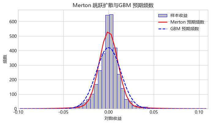

图 1.9 Merton 跳跃扩散模型对 S&P 500 日对数收益率整体分布的拟合。红色实线为 Merton 每箱预期频数，蓝色虚线为GBM 每箱预期频数。

显然Merton扩散跳跃模型对收益分布尾部的拟合比起正态分布有很大改进，但在分布的中心部分的峰态还是不够尖。

以下图 1.9a 和 1.9b 比较 Merton 跳跃扩散模型与 GBM 在左右尾部的拟合。

# 图 1.9a、1.9b：整理左右尾比较使用的直方图频数
tail_bin_edges = fit_bin_edges
tail_bin_centres = (tail_bin_edges[:-1] + tail_bin_edges[1:]) / 2
tail_bin_width = tail_bin_edges[1] - tail_bin_edges[0]
tail_return_grid = np.linspace(
    tail_bin_edges[0], tail_bin_edges[-1], 2000
)
histogram_counts, _ = np.histogram(log_returns, bins=tail_bin_edges)
gbm_expected_counts = (
    norm.pdf(
        tail_return_grid,
        loc=drift * time_step,
        scale=volatility * np.sqrt(time_step),
    )
    * len(log_returns)
    * tail_bin_width
)

绘图辅助函数：模型密度与 GBM 左尾、右尾的比较

def plot_tail_comparison(
    tail_return_grid,
    tail_bin_centres,
    histogram_counts,
    tail_bin_width,
    gbm_expected_counts,
    model_expected_counts,
    model_label,
    x_limits,
    title,
):
    '''Compare observed tail-bin counts with a model and the GBM benchmark.'''
    grid_in_tail = (
        (tail_return_grid >= x_limits[0])
        & (tail_return_grid <= x_limits[1])
    )
    bins_in_tail = (
        (tail_bin_centres >= x_limits[0])
        & (tail_bin_centres <= x_limits[1])
    )
    fig, ax = plt.subplots(figsize=(8, 4.2))
    ax.bar(
        tail_bin_centres[bins_in_tail],
        histogram_counts[bins_in_tail],
        width=tail_bin_width,
        color="0.75",
        edgecolor="blue",
        linewidth=0.8,
        label="样本收益",
    )
    ax.plot(
        tail_return_grid[grid_in_tail],
        model_expected_counts[grid_in_tail],
        color="red",
        linewidth=1.8,
        label=model_label,
    )
    ax.plot(
        tail_return_grid[grid_in_tail],
        gbm_expected_counts[grid_in_tail],
        color="blue",
        linewidth=1.8,
        linestyle="--",
        label="GBM 正态密度",
    )
    ax.set_xlim(*x_limits)
    ax.set_ylim(0.0, 50.0)
    if x_limits[1] <= 0.0:
        ax.set_xticks(np.arange(-0.10, -0.019, 0.02))
    else:
        ax.set_xticks(np.arange(0.02, 0.101, 0.02))
    ax.set_xlabel("每日对数收益")
    ax.set_ylabel("每个区间的观测数")
    ax.set_title(title)
    ax.legend(frameon=False)
    fig.tight_layout()
    return fig

# 图 1.9a：Merton 跳跃扩散与 GBM 在左尾的比较
merton_expected_counts = (
    merton_increment_density(
        tail_return_grid,
        merton_drift,
        merton_diffusion_volatility,
        merton_jump_intensity,
        0.0,
        merton_jump_std,
        time_step,
    )
    * len(log_returns)
    * tail_bin_width
)
plot_tail_comparison(
    tail_return_grid,
    tail_bin_centres,
    histogram_counts,
    tail_bin_width,
    gbm_expected_counts,
    merton_expected_counts,
    "Merton 跳跃扩散",
    (-0.10, -0.02),
    "Merton 跳跃扩散与 GBM：左尾",
)
plt.show()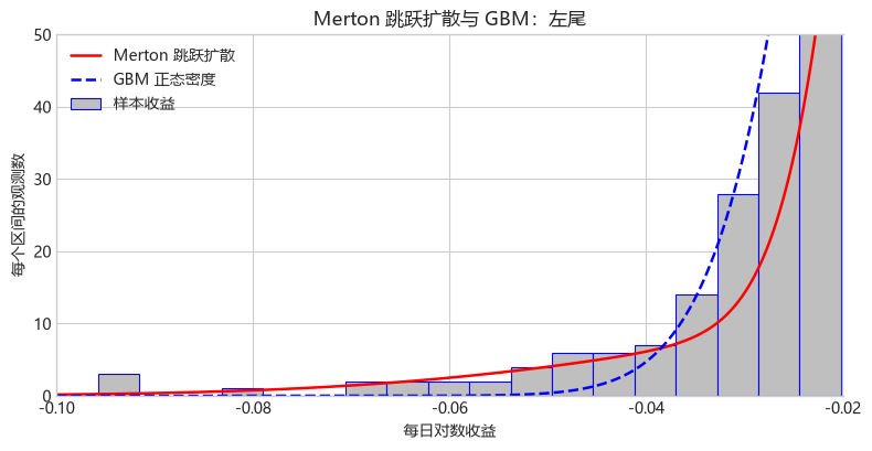

图 1.9a Merton 跳跃扩散模型与 GBM 在左尾的比较。

# 图 1.9b：Merton 跳跃扩散与 GBM 在右尾的比较
plot_tail_comparison(
    tail_return_grid,
    tail_bin_centres,
    histogram_counts,
    tail_bin_width,
    gbm_expected_counts,
    merton_expected_counts,
    "Merton 跳跃扩散",
    (0.02, 0.11),
    "Merton 跳跃扩散与 GBM：右尾",
)
plt.show()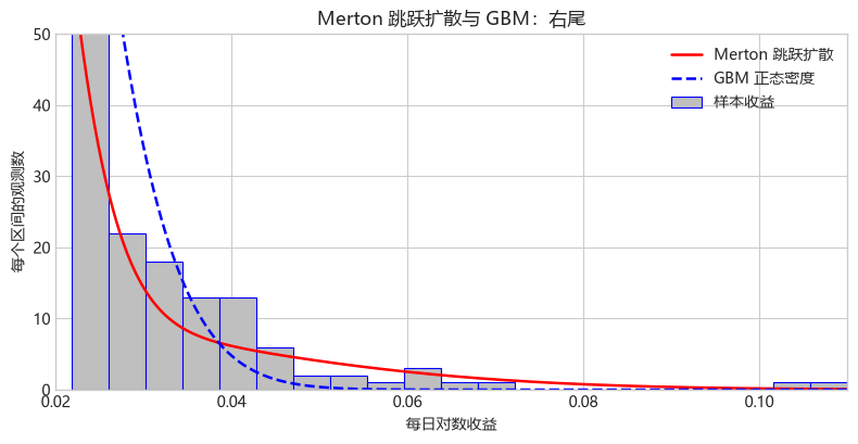

图 1.9b Merton 跳跃扩散模型与 GBM 在右尾的比较。

1.5 方差伽马模型

Variance Gamma模型由 Madan 等（1998）提出。本节将介绍如何用VG过程拟合历史股票收益。

1.5.1 Gamma 分布和 Gamma 过程

记 \(\gamma(t;\mu,\nu)\) 为一 \(Gamma\) 过程，其在 \((t,t+h)\) 的增量 \(g=\gamma(t+h;\mu,\nu)-\gamma(t;\mu,\nu)\) 的概率密度函数是均值为 \(\mu h\)、方差为 \(\nu h\) 的 \(Gamma\) 分布，

\[ f_h(g)=\left(\frac{\mu}{\nu}\right)^{\frac{\mu^2h}{\nu}} \frac{g^{\frac{\mu^2h}{\nu}-1}e^{-\frac{\mu}{\nu}g}} {\Gamma\left(\frac{\mu^2h}{\nu}\right)},\quad g>0. \]

其中 \(\Gamma(\cdot)\) 表示 gamma 函数 \(\Gamma(z)=\int_0^\infty u^{z-1}e^{-u}\,du\)。

# 导入本节所需的计算、统计和绘图库
from scipy.stats import gamma as gamma_distribution
from scipy.special import gammaln, kve

gamma_mean = 1.0
gamma_variance_rate = 0.01
gamma_intervals = [1 / 50, 1 / 250]
gamma_grid = np.linspace(1e-6, 0.10, 500)

公式与代码对应

increment 对应 \(g\)，mean_rate、variance_rate 和 interval 分别对应 \(\mu,\nu,h\)。SciPy 使用形状与尺度参数：shape 对应 \(\mu^2h/\nu\)，scale 对应 \(\nu/\mu\)。

Python程序 1.3：Gamma过程增量密度函数

def gamma_increment_density(increment, mean_rate, variance_rate, interval):
    '''Evaluate a Gamma increment density from its mean and variance rates.'''
    shape = mean_rate**2 * interval / variance_rate
    scale = variance_rate / mean_rate
    return gamma_distribution.pdf(increment, a=shape, scale=scale)

# 图 1.10 左图：计算两个时间间隔下的 Gamma 增量密度
gamma_densities = [
    gamma_increment_density(
        gamma_grid, gamma_mean, gamma_variance_rate, interval
    )
    for interval in gamma_intervals
]

# 图 1.10 右图：设置 Gamma 过程样本路径的时间网格
gamma_path_rng = np.random.default_rng(43)
gamma_path_dt = 1 / 50
gamma_path_steps = int(1 / gamma_path_dt)

程序 1.4 通过累加独立的 Gamma 增量生成样本路径。输入路径数、时间步数和过程参数，返回每个时间点的路径值。

公式与代码对应

increments 的每行对应一条路径，每列对应一个时间步的 Gamma 增量，其均值为 \(\mu h\)、方差为 \(\nu h\)。paths 的首列为初值 \(0\)，后续各列由增量沿时间方向累加得到。

Python程序 1.4：Gamma过程样本路径模拟函数

def gamma_process_paths(
    number_of_paths,
    number_of_steps,
    mean_rate,
    variance_rate,
    time_step,
    rng,
):
    '''Generate Gamma-process paths from independent Gamma increments.

    Each increment has mean mean_rate*time_step and variance
    variance_rate*time_step.
    '''
    shape = mean_rate**2 * time_step / variance_rate
    scale = variance_rate / mean_rate
    increments = rng.gamma(
        shape=shape,
        scale=scale,
        size=(number_of_paths, number_of_steps),
    )
    paths = np.column_stack(
        [np.zeros(number_of_paths), np.cumsum(increments, axis=1)]
    )
    return paths

# 调用程序 1.4 生成十条 Gamma 过程路径
gamma_paths = gamma_process_paths(
    10,
    gamma_path_steps,
    gamma_mean,
    gamma_variance_rate,
    gamma_path_dt,
    gamma_path_rng,
)
gamma_path_time = np.linspace(0.0, 1.0, gamma_path_steps + 1)

图 1.10 左图是对应参数 \(\mu=1,\nu=0.01,h\in\{1/50,1/250\}\) 的 Gamma 分布概率密度函数。由于 Gamma 分布的定义域为 \((0,+\infty)\)，所以 Gamma 过程是一个递增的过程，如图 1.10 右图所示。

# 图 1.10：参数为 $\mu=1$、$\nu=0.01$ 且 $h\in\{1/50,1/250\}$ 时的 Gamma 密度（左）和 Gamma 过程的 10 条样本路径（右）
fig, axes = plt.subplots(1, 2, figsize=(11, 4.3))
for interval, density in zip(gamma_intervals, gamma_densities):
    axes[0].plot(gamma_grid, density, label=fr"$h={interval:g}$")
axes[0].set_xlabel("Gamma 增量")
axes[0].set_ylabel("密度")
axes[0].set_title("Gamma 增量密度")
axes[0].grid(True, alpha=0.25)
axes[0].set_ylim(0.0, 160.0)
axes[0].legend()
axes[1].plot(gamma_path_time, gamma_paths.T, alpha=0.22)
axes[1].set_xlabel("时间")
axes[1].set_ylabel(r"$\gamma(t)$")
axes[1].set_title("Gamma 过程样本路径")
axes[1].grid(True, alpha=0.25)
fig.tight_layout()
plt.show()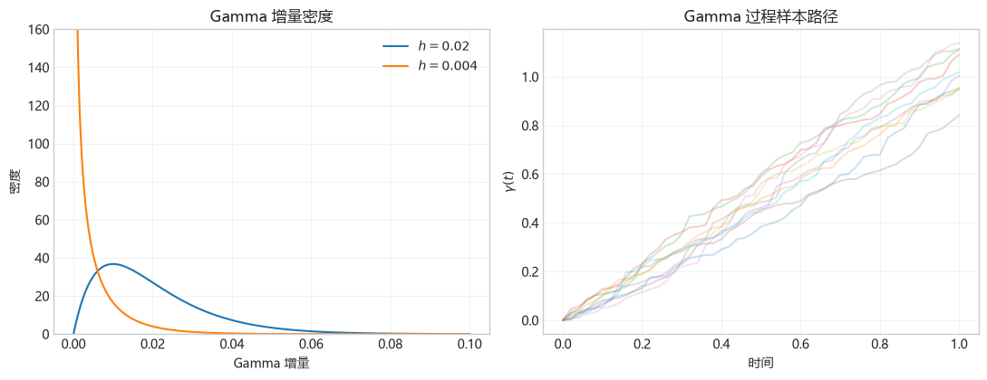

图 1.10 对应参数 \(\mu=1,\nu=0.01,h\in\{1/50,1/250\}\) 的 Gamma 分布概率密度和 Gamma 过程的样本路径。

1.5.2 Variance Gamma 过程

记 \(b(t;\theta,\sigma)=\theta t+\sigma W(t)\) 为漂移率为 \(\theta\)、波动率为 \(\sigma\) 的布朗运动。如果把 \(b(t)\) 中的日历时间 \(t\) 替换为由 \(\gamma(t;1,\nu)\) 过程给出的随机时间，也就是

\[ X_t(\sigma,\nu,\theta)=b(\gamma(t;1,\nu);\theta,\sigma). \]

我们就得到 Variance Gamma 过程，以后简称为 VG 过程。VG 过程的三个参数中，\(\theta\) 主要控制分布的偏度，而 \(\nu\) 主要控制分布的峰度。

因为 Gamma 路径始终递增，可以把 \(G_t=\gamma(t;1,\nu)\) 理解为业务时钟。虽然每个交易日的日历长度相同，但市场处理的信息量、交易活跃程度和价格波动强弱可能差别很大。例如，公司发布季报后，市场可能在一天内集中处理更多信息；业务时钟的比喻，就是把这样的交易日理解为时钟走得较快。市场活动越密集，同一段日历时间内业务时钟前进得通常越多，而平静的市场则对应较慢的业务时钟。因此，随机业务时钟可带来每步条件标准差的随机变化。对于 GBM，每步对数收益的标准差为 \(\sigma\sqrt{h}\)；对于 VG，给定本步的 Gamma 时钟增量 \(g\) 后，

\[ \Delta X\mid\Delta G=g\sim\mathcal{N}(\theta g,\sigma^2g), \qquad \operatorname{SD}(\Delta X_{\mathrm{GBM}})=\sigma\sqrt{h}, \quad \operatorname{SD}(\Delta X_{\mathrm{VG}}\mid\Delta G=g)=\sigma\sqrt{g}. \]

所以在相同长度的日历时间步中，GBM 的每步标准差固定；VG 的每步条件标准差则随 Gamma 增量而变化。下表以 \(h=0.2\)、\(\theta=0\)、\(\sigma=0.25\)、\(\nu=0.1\) 为例，列出五个独立的 Gamma 增量 \(\Delta G_i\sim\operatorname{Gamma}(h/\nu,\text{scale}=\nu)=\operatorname{Gamma}(2,0.1)\)。

时间步	\(\Delta G_i\)	GBM 每步标准差 \(\sigma\sqrt{h}\)	VG 条件标准差 \(\sigma\sqrt{\Delta G_i}\)
1	0.2482	0.1118	0.1246
2	0.1456	0.1118	0.0954
3	0.3331	0.1118	0.1443
4	0.2963	0.1118	0.1361
5	0.1519	0.1118	0.0974

表 1.2 相同日历时间步下，GBM 每步标准差与 VG 每步条件标准差的比较。

表中的 VG 数值是给定 Gamma 增量后的条件标准差；对 Gamma 随机性取平均后，增量的无条件方差为 \(\operatorname{Var}(\Delta X)=(\sigma^2+\theta^2\nu)h\)。本例 \(\theta=0\)，所以无条件方差仍为 \(\sigma^2h\)。

记 \(X_h=X_{t+h}-X_t\) 为 \(X_t\) 在时间 \(h>0\) 的增量。业务时钟增量 \(G_h\) 服从形状参数为 \(h/\nu\)、尺度参数为 \(\nu\) 的 Gamma 分布，给定 \(G_h=g\) 后，\(X_h\) 服从均值为 \(\theta g\)、方差为 \(\sigma^2g\) 的正态分布。因此，VG 增量密度首先可以写成正态密度关于 Gamma 时钟的混合积分：

\[ \begin{aligned} p_h(x) &=\int_0^{+\infty} \frac{1}{\sqrt{2\pi\sigma^2g}} \exp\!\left(-\frac{(x-\theta g)^2}{2\sigma^2g}\right) \frac{g^{h/\nu-1}e^{-g/\nu}} {\nu^{h/\nu}\Gamma(h/\nu)}\,dg. \end{aligned} \]

将 Gamma 时钟积分掉后，可以把该混合密度化为以下闭式表达式：

\[ \begin{aligned} p_h(x)=\frac{\sqrt{2}e^{\theta x/\sigma^2}} {\sigma\sqrt{\pi}\nu^{h/\nu}\Gamma(h/\nu)} \left(\frac{|x|}{\sqrt{2\sigma^2/\nu+\theta^2}}\right)^{h/\nu-1/2} K_{h/\nu-1/2}\left(\frac{|x|\sqrt{2\sigma^2/\nu+\theta^2}} {\sigma^2}\right). \end{aligned} \tag{1.5.1} \]

其中 \(K_v\) 表示 \(v\) 阶第二类修正贝塞尔函数（modified Bessel function of the second kind），是修正贝塞尔常微分方程的解；式（1.5.1）中的阶数为 \(v=h/\nu-1/2\)。

该贝塞尔表达式在 \(x=0\) 处应取极限：当 \(h/\nu>1/2\) 时密度有限；当 \(h/\nu\leq1/2\) 时密度趋于正无穷，但这一奇点可积，分布仍然具有有限的总概率。

\(X_h\) 的均值及二至四阶中心矩分别为

\[ \mu_1=E[X_h]=\theta h \tag{1.5.2} \]

\[ \mu_2=E[(X_h-E[X_h])^2]=(\theta^2\nu+\sigma^2)h \tag{1.5.3} \]

\[ \mu_3=E[(X_h-E[X_h])^3]=(2\theta^3\nu^2+3\sigma^2\theta\nu)h \tag{1.5.4} \]

\[ \mu_4=E[(X_h-E[X_h])^4] =(3\sigma^4\nu+12\sigma^2\theta^2\nu^2+6\theta^4\nu^3)h+3\mu_2^2 \tag{1.5.5} \]

VG 过程也可以被表示为两个独立的 \(Gamma\) 过程的差，这将在第 3.2.4.3 节介绍。

1.5.3 VG 模型的矩估计

接下来我们介绍如何通过带漂移的 VG 模型

\[ X_t=ct+b(\gamma(t;1,\nu);\theta,\sigma) \tag{1.5.6} \]

来拟合历史股票收益。加入漂移项 \(ct\) 后，\(X\) 在时间 \([t,t+h]\) 的增量 \(X_h=X_{t+h}-X_t\) 的概率密度函数为 \(f_h(x)=p_h(x-ch)\)（其中 \(p_h(\cdot)\) 已由式（1.5.1）给出），可由 Python 程序 1.5 计算。程序在 \(x=ch\) 处使用密度的中心极限，在其他位置计算贝塞尔表达式。

公式与代码对应

centred 对应 \(x-ch\)，shape 对应 \(h/\nu\)，scale_squared 对应 \(2\sigma^2/\nu+\theta^2\)。argument 是贝塞尔函数的自变量。

SciPy 的 kve 返回 \(e^zK_v(z)\)，因此代码用 \(\log(\operatorname{kve}(v,z))-z\) 计算 \(\log K_v(z)\)；这里的 \(z\) 就是 argument。

Python程序 1.5：Variance Gamma增量密度函数

def variance_gamma_increment_density(
    x, sigma, nu, theta, c, time_step
):
    '''Evaluate the VG increment density at x.

    The parameters are the Brownian volatility sigma, Gamma-clock
    variance rate nu, Brownian drift theta, deterministic drift c,
    and interval length time_step.
    '''
    centred = np.asarray(x, dtype=float) - c * time_step
    shape = time_step / nu
    scale_squared = 2.0 * sigma**2 / nu + theta**2
    absolute_centred = np.where(centred == 0, 1.0, np.abs(centred))
    argument = absolute_centred * np.sqrt(scale_squared) / sigma**2
    power = shape / 2.0 - 0.25
    log_density = (
        np.log(2.0)
        + theta * centred / sigma**2
        - shape * np.log(nu)
        - np.log(sigma)
        - 0.5 * np.log(2.0 * np.pi)
        - gammaln(shape)
        + power
        * (2.0 * np.log(absolute_centred) - np.log(scale_squared))
        + np.log(kve(shape - 0.5, argument))
        - argument
    )
    density = np.exp(log_density)
    if shape > 0.5:
        centre_density = np.exp(
            gammaln(shape - 0.5) - gammaln(shape)
            - np.log(sigma) - 0.5 * np.log(2.0 * np.pi * nu)
            - (shape - 0.5) * np.log(1.0 + theta**2 * nu / (2.0 * sigma**2))
        )
    else:
        centre_density = np.inf  # An integrable density singularity.
    return np.where(centred == 0, centre_density, density)

Figueroa-López 等（2011）提供了 VG 过程的矩估计。注意由于我们加入了漂移项 \(ct\)，所以 \(X_h\) 的一阶矩需要修正为

\[ \mu_1=E[X_h]=(\theta+c)h \tag{1.5.7} \]

因为 \(c\) 是常数，不具有随机性，所以不改变 \(X_h\) 的二至四阶中心矩。因此，VG 模型（1.5.6）的矩估计需要求解式（1.5.3）、式（1.5.4）、式（1.5.5）和式（1.5.7）。

首先计算样本的四阶矩

\[ \hat\mu_{1,n}=\frac{1}{n}\sum_{i=1}^n x_i=(\hat\theta+\hat c)h \tag{1.5.8} \]

\[ \hat\mu_{k,n}=\frac{1}{n}\sum_{i=1}^n \left(x_i-\hat\mu_{1,n}\right)^k,\quad k=2,3,4 \tag{1.5.9} \]

然后计算样本的方差、偏度和峰度

\[ \widehat{Var}_n=\frac{1}{n}\sum_{i=1}^n(x_i-\bar{x})^2 \tag{1.5.10} \]

\[ \widehat{Skw}_n=\frac{\hat\mu_{3,n}}{\hat\mu_{2,n}^{3/2}} \tag{1.5.11} \]

\[ \widehat{Krt}_n=\frac{\hat\mu_{4,n}}{\hat\mu_{2,n}^2}-3 \tag{1.5.12} \]

定义无量纲参数 \(\xi=\theta^2\nu/\sigma^2\)，它表示 Gamma 时钟中的随机漂移对方差的贡献与布朗随机部分方差贡献之比。接下去用数值方法求解其估计值 \(\xi^*\)，满足

\[ \frac{\xi(3+2\xi)^2}{(1+4\xi+2\xi^2)(1+\xi)} =\frac{3\widehat{Skw}_n^2}{\widehat{Krt}_n} \tag{1.5.13} \]

最后 VG 模型的四个参数可以由以下表达式给出

\[ \hat\sigma_n^2=\frac{\widehat{Var}_n}{h} \left(\frac{1}{1+\xi^*}\right) \tag{1.5.14} \]

\[ \hat\nu=\frac{h}{3}\widehat{Krt}_n \left(\frac{(1+\xi^*)^2}{1+4\xi^*+2(\xi^*)^2}\right) \tag{1.5.15} \]

\[ \hat\theta=\frac{\hat\mu_{3,n}} {h\hat{\sigma}^2\hat\nu} \left(\frac{1}{3+2\xi^*}\right) \tag{1.5.16} \]

\[ \hat{c}=\frac{1}{h}\bar{x}-\hat\theta =\frac{\sum_{i=1}^n x_i}{T}-\hat\theta \tag{1.5.17} \]

VG 模型的矩估计可以由 Python 程序 1.6 计算。

当样本超额峰度 \(\widehat{Krt}_n>0\)，且 \(0\leq3\widehat{Skw}_n^2/\widehat{Krt}_n<2\) 时，式（1.5.13）有唯一的有限非负解 \(\xi^*\)。这是因为左侧比值函数在 \(\xi\geq0\) 上严格递增，取值范围为 \([0,2)\)。

# 导入本节所需的方程求解工具
from scipy.optimize import root_scalar

公式与代码对应

比值函数的 value 对应 \(\xi\)，矩估计函数中的 xi_star 对应求得的 \(\xi^*\)。sample_excess_kurtosis 保存超额峰度，target 对应 \(3\widehat{\operatorname{Skew}}^2/\widehat{\operatorname{Kurt}}_{\rm excess}\)。

Python程序 1.6：Variance Gamma矩估计中的无量纲比值函数、Variance Gamma模型累积量矩估计函数

def vg_moment_ratio(value):
    '''Return the dimensionless VG moment ratio in the xi equation.'''
    return value * (3 + 2 * value) ** 2 / (
        (1 + 4 * value + 2 * value**2) * (1 + value)
    )


def fit_variance_gamma_moments(log_returns, time_step):
    '''Estimate VG parameters from sample moments and cumulants.'''
    sample_mean = np.mean(log_returns)
    sample_variance = np.var(log_returns, ddof=0)
    sample_skewness = skew(log_returns, bias=True)
    sample_excess_kurtosis = kurtosis(
        log_returns, fisher=True, bias=True
    )
    target = 3 * sample_skewness**2 / sample_excess_kurtosis
    root_result = root_scalar(
        lambda value: vg_moment_ratio(value) - target,
        bracket=(0.0, 1.0e6),
        method="brentq",
    )
    xi_star = root_result.root
    sigma = np.sqrt(sample_variance / (time_step * (1 + xi_star)))
    nu = (
        time_step
        / 3
        * sample_excess_kurtosis
        * (1 + xi_star) ** 2
        / (1 + 4 * xi_star + 2 * xi_star**2)
    )
    theta = (
        sample_skewness
        * sample_variance**1.5
        / (time_step * sigma**2 * nu * (3 + 2 * xi_star))
    )
    c = sample_mean / time_step - theta
    return sigma, nu, theta, c

# 调用程序 1.6 估计 Variance Gamma 模型参数
vg_sigma, vg_nu, vg_theta, vg_c = fit_variance_gamma_moments(
    log_returns, time_step
)
vg_parameters = pd.Series(
    {"sigma": vg_sigma, "nu": vg_nu, "theta": vg_theta, "c": vg_c},
    name="VG 矩估计",
)
vg_parameters

sigma    0.211462
nu       0.009873
theta   -0.075602
c        0.082927
Name: VG 矩估计, dtype: float64

# 将 VG 密度在统一分箱内积分，中心奇点单独作为积分分割点
vg_hist_edges = fit_bin_edges
vg_bin_centres = fit_bin_centres
vg_bin_counts = model_bin_counts(
    lambda x: variance_gamma_increment_density(
        x, vg_sigma, vg_nu, vg_theta, vg_c, time_step
    ), centre=vg_c * time_step
)
vg_expected_counts = vg_bin_counts
vg_normal_counts = normal_bin_counts

VG 模型的矩估计为

\[ \hat\theta=-0.075602,\quad\hat\nu=0.009873, \quad\hat\sigma=0.211462,\quad\hat c=0.082927 \tag{1.5.18} \]

图 1.11 中红色实线为 VG 模型每箱预期频数，蓝色虚线为 GBM 的对应结果。

# 图 1.11：Variance Gamma 模型对 S&P 500 日对数收益率整体分布的拟合。红色实线为 VG 预期频数，蓝色虚线为GBM 预期频数
fig, ax = plt.subplots(figsize=(8, 4.2))
ax.hist(log_returns, bins=vg_hist_edges, alpha=0.35, label="样本收益")
ax.plot(
    vg_bin_centres,
    vg_expected_counts,
    color="tab:red",
    label="VG 预期频数",
)
ax.plot(
    vg_bin_centres,
    vg_normal_counts,
    color="tab:blue",
    linestyle="--",
    label="GBM 预期频数",
)
ax.set_xlim(fit_bin_edges[0], fit_bin_edges[-1])
ax.set_xlabel("对数收益")
ax.set_ylabel("频数")
ax.set_title("Variance Gamma 拟合")
ax.legend()
plt.show()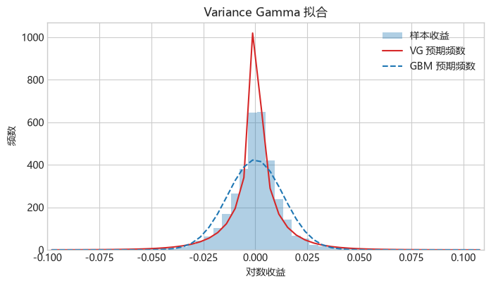

图 1.11 VG 模型拟合的 2000 年 1 月至 2013 年 6 月 S&P 500 指数的对数收益，其中红色实线为拟合的 VG 模型的每箱预期频数，而蓝色虚线为相应的GBM结果。两条曲线均按直方图的区间换算为预期频数。

显然VG模型对收益分布尾部的拟合比起正态分布有很大改进，但在分布的中心部分的尖峰过高。

以下图1.11a 和 1.11b 比较 VG 模型与 GBM 在左右尾部的拟合。

# 图 1.11a：Variance Gamma 与 GBM 在左尾的比较
vg_expected_counts = (
    variance_gamma_increment_density(
        tail_return_grid,
        vg_sigma,
        vg_nu,
        vg_theta,
        vg_c,
        time_step,
    )
    * len(log_returns)
    * tail_bin_width
)
plot_tail_comparison(
    tail_return_grid,
    tail_bin_centres,
    histogram_counts,
    tail_bin_width,
    gbm_expected_counts,
    vg_expected_counts,
    "Variance Gamma",
    (log_returns.min(), -0.02),
    "Variance Gamma 与 GBM：左尾",
)
plt.show()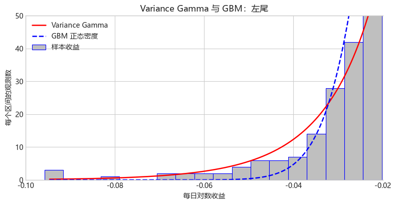

图 1.11a Variance Gamma 模型与 GBM 在左尾的比较。

# 图 1.11b：Variance Gamma 与 GBM 在右尾的比较
plot_tail_comparison(
    tail_return_grid,
    tail_bin_centres,
    histogram_counts,
    tail_bin_width,
    gbm_expected_counts,
    vg_expected_counts,
    "Variance Gamma",
    (0.02, log_returns.max()),
    "Variance Gamma 与 GBM：右尾",
)
plt.show()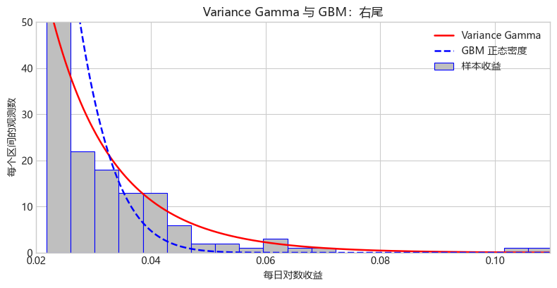

图 1.11b Variance Gamma 模型与 GBM 在右尾的比较。

1.6 正态逆高斯模型

Normal Inverse Gaussian（NIG）过程由 Barndorff-Nielsen（1997）提出。本节将介绍如何用 NIG 过程拟合历史股票收益。

1.6.1 逆高斯过程

记 \(IG(t;\mu,\lambda)\) 为 Inverse Gaussian（IG）过程。其在 \((t,t+h)\) 的增量 \(g=IG(t+h;\mu,\lambda)-IG(t;\mu,\lambda)\) 服从 Inverse Gaussian 分布，

\[ f_h(g;\mu,\lambda)= \sqrt{\frac{\lambda h^2}{2\pi g^3}} \exp\left[-\frac{\lambda(g-\mu h)^2}{2\mu^2g}\right], \quad g>0 \tag{1.6.1} \]

\(\mu>0\) 是均值率，增量均值为 \(E[g]=\mu h\)；\(\lambda>0\) 是形状率，增量的形状参数为 \(\lambda h^2\)，方差为 \(\operatorname{Var}(g)=\mu^3h/\lambda\)。本章用于 NIG 时钟时取 \(\mu=1\)、\(\lambda=1/\nu\)，因此增量均值为 \(h\)、方差为 \(\nu h\)。下面计算 \(\mu=1\)、\(\nu=0.01\) 且 \(h\in\{1/50,1/250\}\) 时的密度，并模拟 \(T=1\) 的样本路径。

# 导入本节所需的计算、统计和绘图库
from scipy.stats import invgauss

inverse_gaussian_mean = 1.0
inverse_gaussian_shape = 1.0 / 0.01
inverse_gaussian_intervals = [1 / 50, 1 / 250]
inverse_gaussian_grid = np.linspace(1e-4, 0.14, 500)

公式与代码对应

mean_increment 对应 \(\mu h\)，shape_increment 对应 \(\lambda h^2\)。调用 SciPy 的逆高斯密度时，scipy_shape 为两者之比，并将 shape_increment 传给尺度参数。

Python程序 1.7：逆高斯增量密度函数

def inverse_gaussian_increment_density(
    increment, mean_rate, shape_rate, interval
):
    '''Evaluate an inverse-Gaussian increment density.

    SciPy's inverse-Gaussian parameter mu is the ratio of the mean
    parameter to the scale parameter, while scale carries the
    interval-dependent shape parameter.
    '''
    mean_increment = mean_rate * interval
    shape_increment = shape_rate * interval**2
    scipy_shape = mean_increment / shape_increment
    return invgauss.pdf(
        increment, mu=scipy_shape, scale=shape_increment
    )

# 图 1.12 左图：计算两个时间间隔下的逆高斯增量密度
inverse_gaussian_densities = [
    inverse_gaussian_increment_density(
        inverse_gaussian_grid,
        inverse_gaussian_mean,
        inverse_gaussian_shape,
        interval,
    )
    for interval in inverse_gaussian_intervals
]

# 图 1.12 右图：设置逆高斯过程样本路径的时间网格
inverse_gaussian_path_rng = np.random.default_rng(44)
inverse_gaussian_path_dt = 1 / 50
inverse_gaussian_path_steps = int(1 / inverse_gaussian_path_dt)

程序 1.8 通过累加独立的逆高斯增量生成样本路径。输入路径数、时间步数和过程参数，返回每个时间点的路径值。

公式与代码对应

NumPy 的 rng.wald 直接接收逆高斯分布的均值 \(\mu h\) 和形状参数 \(\lambda h^2\)。increments 按行保存各条路径的增量；paths 在首列放置 \(0\)，再沿时间方向累加。

Python程序 1.8：逆高斯过程样本路径模拟函数

def inverse_gaussian_process_paths(
    number_of_paths,
    number_of_steps,
    mean_rate,
    shape_rate,
    time_step,
    rng,
):
    '''Generate inverse-Gaussian-process paths.

    NumPy's wald sampler uses mean=mean_rate*time_step and
    scale=shape_rate*time_step**2 for each increment.
    '''
    increments = rng.wald(
        mean=mean_rate * time_step,
        scale=shape_rate * time_step**2,
        size=(number_of_paths, number_of_steps),
    )
    return np.column_stack(
        [np.zeros(number_of_paths), np.cumsum(increments, axis=1)]
    )

# 图 1.12 右图：调用程序 1.8 生成十条逆高斯过程路径
inverse_gaussian_paths = inverse_gaussian_process_paths(
    10,
    inverse_gaussian_path_steps,
    inverse_gaussian_mean,
    inverse_gaussian_shape,
    inverse_gaussian_path_dt,
    inverse_gaussian_path_rng,
)
inverse_gaussian_path_time = np.linspace(
    0.0, 1.0, inverse_gaussian_path_steps + 1
)

图 1.12 左图是对应参数 \(\mu=1,\nu=0.01,h\in\{1/50,1/250\}\) 的 Inverse Gaussian（IG）分布概率密度函数。由于 IG 分布的定义域为 \((0,+\infty)\)，所以 IG 过程是一个递增的过程，如图 1.12 右图所示。

# 图 1.12：参数为 $\mu=1$、$\nu=0.01$ 且 $h\in\{1/50,1/250\}$ 时的逆高斯密度（左）和逆高斯过程的 10 条样本路径（右）
fig, axes = plt.subplots(1, 2, figsize=(11, 4.3))
for interval, density in zip(
    inverse_gaussian_intervals, inverse_gaussian_densities
):
    axes[0].plot(
        inverse_gaussian_grid,
        density,
        label=fr"$h={interval:g}$",
    )
axes[0].set_xlabel("逆高斯增量")
axes[0].set_ylabel("密度")
axes[0].set_title("逆高斯增量密度")
axes[0].grid(True, alpha=0.25)
axes[0].set_ylim(0.0, 300.0)
axes[0].legend()
axes[1].plot(
    inverse_gaussian_path_time,
    inverse_gaussian_paths.T,
    alpha=0.22,
)
axes[1].set_xlabel("时间")
axes[1].set_ylabel("$IG(t)$")
axes[1].set_title("逆高斯过程样本路径")
axes[1].grid(True, alpha=0.25)
fig.tight_layout()
plt.show()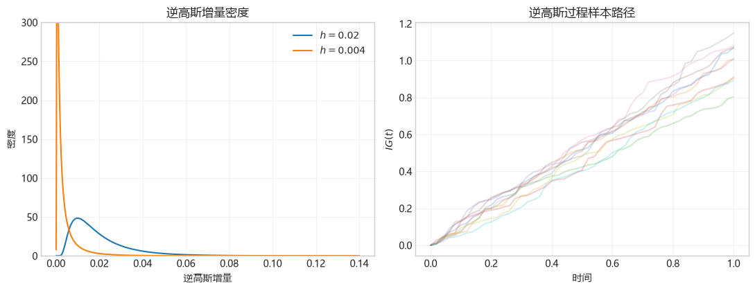

图 1.12 参数为 \(\mu=1\)、\(\nu=0.01\) 且 \(h\in\{1/50,1/250\}\) 时的逆高斯密度（左）和逆高斯过程的 10 条样本路径（右）。

1.6.2 正态逆高斯过程

设布朗运动与逆高斯时钟相互独立。如果把漂移率为 \(\theta\)、波动率为 \(\sigma\) 的布朗运动 \(b(t;\theta,\sigma)=\theta t+\sigma W(t)\) 中的日历时间 \(t\) 替换为由 \(IG(t;1,1/\nu)\) 过程给出的随机时间，也就是

\[ X(t;\sigma,\nu,\theta)=b(IG(t;1,1/\nu);\theta,\sigma). \]

我们就得到 Normal Inverse Gaussian 过程，以后简称为 NIG 过程。

NIG 与 VG 的时间变换构造相同：布朗运动按业务时间运行，观察者按日历时间看路径；区别在于 NIG 使用逆高斯时钟，而 VG 使用 Gamma 时钟。若 \(H_h=IG(t+h;1,1/\nu)-IG(t;1,1/\nu)\)，给定 \(H_h=g\) 时，基本 NIG 过程的增量仍服从 \(\mathcal{N}(\theta g,\sigma^2g)\)；加入确定性漂移 \(ct\) 后，条件均值同样变为 \(ch+\theta g\)。在本章的参数化下，两种时钟的增量都有均值 \(h\) 和方差 \(\nu h\)，但其分布不同，因此对条件正态分布的混合也不同，产生不同的非正态收益分布。

记 \(X_h=X_{t+h}-X_t\) 为 \(X_t\) 在时间 \(h>0\) 的增量。\(X_h\) 的概率密度函数由式（1.6.2）给出，

\[ \begin{aligned} p_h(x)=\frac{h e^{h/\nu+\theta x/\sigma^2}}{\pi} \left(\frac{x^2+h^2\sigma^2/\nu} {\theta^2/(\nu\sigma^2)+1/\nu^2}\right)^{-1/2} K_1\left(\frac{\sqrt{x^2+h^2\sigma^2/\nu} \sqrt{\sigma^2/\nu+\theta^2}}{\sigma^2}\right). \end{aligned} \tag{1.6.2} \]

而 \(X_h\) 的均值及二至四阶中心矩分别为

\[ \mu_1=E[X_h]=\theta h \tag{1.6.3} \]

\[ \mu_2=E[(X_h-E[X_h])^2]=(\theta^2\nu+\sigma^2)h \tag{1.6.4} \]

\[ \mu_3=E[(X_h-E[X_h])^3]=(3\theta^3\nu^2+3\sigma^2\theta\nu)h \tag{1.6.5} \]

\[ \mu_4=E[(X_h-E[X_h])^4] =(3\sigma^4\nu+18\sigma^2\theta^2\nu^2+15\theta^4\nu^3)h+3\mu_2^2 \tag{1.6.6} \]

Barndorff-Nielsen（1997）和 Schoutens（2003）还给出了另外一种 NIG 过程的参数设置，我们将在第 3.2.5.3 节介绍如何将这两种参数设置进行转换。

1.6.2.1 NIG 过程的广义矩估计

接下来我们用带漂移的 NIG 模型

\[ X_t=ct+b(IG(t;1,1/\nu);\theta,\sigma) \tag{1.6.7} \]

来拟合 S&P 500 指数。加入漂移项后，\(X\) 在时间 \([t,t+h]\) 的增量 \(X_h=X_{t+h}-X_t\) 的概率密度函数为 \(f_h(x)=p_h(x-ch)\)（其中 \(p_h(\cdot)\) 已由式（1.6.2）给出），可由 Python 程序 1.9a 计算。

密度函数中的 centred 对应 \(x-ch\)，alpha、beta 和 delta 对应转换后的参数，其中 delta 已包含增量长度 \(h\)：\(\delta=\sigma h/\sqrt\nu\)。distance 对应 \(\sqrt{\delta^2+(x-ch)^2}\)。

Python程序 1.9a：Normal Inverse Gaussian增量密度函数

def nig_increment_density(x, sigma, nu, theta, c, time_step):
    '''Evaluate the NIG increment density using its Bessel form.'''
    centred = np.asarray(x, dtype=float) - c * time_step
    alpha = np.sqrt(theta**2 + sigma**2 / nu) / sigma**2
    beta = theta / sigma**2
    delta = sigma * time_step / np.sqrt(nu)
    gamma = np.sqrt(alpha**2 - beta**2)
    distance = np.sqrt(delta**2 + centred**2)
    argument = alpha * distance
    log_density = (
        np.log(alpha * delta / np.pi)
        - np.log(distance)
        + delta * gamma
        + beta * centred
        + np.log(kve(1.0, argument))
        - argument
    )
    return np.exp(log_density)

和 VG 模型类似，由于我们加入了漂移项 \(ct\)，所以 \(X_h=X_{t+h}-X_t\) 的一阶矩需要修正为

\[ \mu_1=E[X_h]=(\theta+c)h \tag{1.6.8} \]

因为 \(c\) 是常数，不具有随机性，所以不改变 \(X_h\) 的二至四阶中心矩。因此，NIG 模型（1.6.7）的矩估计需要求解式（1.6.4）、式（1.6.5）、式（1.6.6）和式（1.6.8）。

首先计算样本的四阶矩

\[ \hat\mu_{1,n}=\frac{1}{n}\sum_{i=1}^n x_i=(\hat\theta+\hat c)h \tag{1.6.9} \]

\[ \hat\mu_{k,n}=\frac{1}{n}\sum_{i=1}^n \left(x_i-\hat\mu_{1,n}\right)^k,\quad k=2,3,4 \tag{1.6.10} \]

然后计算样本的方差、偏度和峰度

\[ \widehat{\operatorname{Var}}_n=\frac{1}{n} \sum_{i=1}^n(x_i-\bar{x})^2 \tag{1.6.11} \]

\[ \widehat{\operatorname{Skew}}_n=\frac{\hat\mu_{3,n}} {\hat\mu_{2,n}^{3/2}} \tag{1.6.12} \]

\[ \widehat{\operatorname{Kurt}}_{\rm excess,n}=\frac{\hat\mu_{4,n}} {\hat\mu_{2,n}^2}-3 \tag{1.6.13} \]

这里仍定义 \(\xi=\theta^2\nu/\sigma^2\)，与 VG 中相同；由于两种时钟的三、四阶累积量不同，求其估计值 \(\xi^*\) 的公式不同：

\[ \xi^*=\frac{\widehat{\operatorname{Skew}}^2} {3\widehat{\operatorname{Kurt}}_{\rm excess} -5\widehat{\operatorname{Skew}}^2} \tag{1.6.14} \]

最后 NIG 模型的四个参数可以由以下表达式给出

\[ \hat\sigma^2=\frac{\widehat{\operatorname{Var}}_n}{h(1+\xi^*)}, \qquad \hat\sigma_n^2=\hat\sigma^2 \tag{1.6.15} \]

\[ \hat\nu=\frac{h}{3}\widehat{\operatorname{Kurt}}_{\rm excess,n} \frac{1+\xi^*}{1+5\xi^*}, \qquad \hat\nu_n=\hat\nu \tag{1.6.16} \]

\[ \hat\theta_n=\frac{\hat\mu_{3,n}} {h\hat\sigma_n^2\hat\nu_n}\frac{1}{3+3\xi^*} \tag{1.6.17} \]

\[ \hat c=\frac{\widehat\mu_{1,n}}{h}-\hat\theta_n =\frac{1}{h}\bar{x}-\hat\theta_n =\frac{\sum_{i=1}^n x_i}{T}-\hat\theta_n \tag{1.6.18} \]

NIG 模型的矩估计可以由 Python 程序 1.9b 计算。

NIG 矩估计要求样本超额峰度为正，并满足 \(3\widehat{\operatorname{Kurt}}_{\rm excess}>5\widehat{\operatorname{Skew}}^2\)，这样才能得到有限、非负的 \(\xi^*\) 和正的 \(\hat\nu\)。

矩估计函数中的 xi_star 对应式（1.6.14）的 \(\xi^*\)；返回的 sigma、nu、theta 和 c 对应四个模型参数的估计值。

Python程序 1.9b：Normal Inverse Gaussian模型累积量矩估计函数

def fit_nig_moments(log_returns, time_step):
    '''Estimate NIG parameters from the sample moments.'''
    sample_mean = np.mean(log_returns)
    sample_variance = np.var(log_returns, ddof=0)
    central_moment_3 = np.mean((log_returns - sample_mean) ** 3)
    sample_skewness = skew(log_returns, bias=True)
    sample_excess_kurtosis = kurtosis(
        log_returns, fisher=True, bias=True
    )
    xi_star = sample_skewness**2 / (
        3 * sample_excess_kurtosis - 5 * sample_skewness**2
    )
    sigma = np.sqrt(sample_variance / (time_step * (1 + xi_star)))
    nu = (
        time_step
        / 3
        * sample_excess_kurtosis
        * (1 + xi_star)
        / (1 + 5 * xi_star)
    )
    theta = central_moment_3 / (
        3 * (1 + xi_star) * time_step * sigma**2 * nu
    )
    c = sample_mean / time_step - theta
    return sigma, nu, theta, c

# 调用程序 1.9b 估计 NIG 模型参数
nig_sigma, nig_nu, nig_theta, nig_c = fit_nig_moments(log_returns, time_step)
nig_parameters = pd.Series(
    {"sigma": nig_sigma, "nu": nig_nu, "theta": nig_theta, "c": nig_c},
    name="NIG 矩估计",
)
nig_parameters

sigma    0.211462
nu       0.009848
theta   -0.075761
c        0.083086
Name: NIG 矩估计, dtype: float64

NIG 模型的矩估计为

\[ \hat\sigma=0.211462,\quad\hat\nu=0.009848, \quad\hat\theta=-0.075761,\quad\hat c=0.083086 \tag{1.6.19} \]

图 1.13 使用与前三种模型相同的分箱：红色实线为 NIG 每箱预期频数，蓝色虚线为 GBM 的对应结果。第 1.6 节末的定量比较进一步汇总中心及尾部拟合。

# 图 1.13：正态逆高斯模型对 S&P 500 日对数收益率整体分布的拟合。红色实线为 NIG 预期频数，蓝色虚线为GBM 预期频数
nig_grid = fit_bin_centres
nig_bin_counts = model_bin_counts(
    lambda x: nig_increment_density(
        x, nig_sigma, nig_nu, nig_theta, nig_c, time_step
    )
)
fig, ax = plt.subplots(figsize=(8, 4.2))
ax.hist(log_returns, bins=fit_bin_edges, alpha=0.35, label="样本收益")
ax.plot(
    nig_grid,
    nig_bin_counts,
    color="tab:red",
    label="NIG 预期频数",
)
ax.plot(
    nig_grid,
    normal_bin_counts,
    color="tab:blue",
    linestyle="--",
    label="GBM 预期频数",
)
ax.set_xlim(fit_bin_edges[0], fit_bin_edges[-1])
ax.set_xlabel("对数收益")
ax.set_ylabel("频数")
ax.set_title("Normal Inverse Gaussian 拟合")
ax.legend()
plt.show()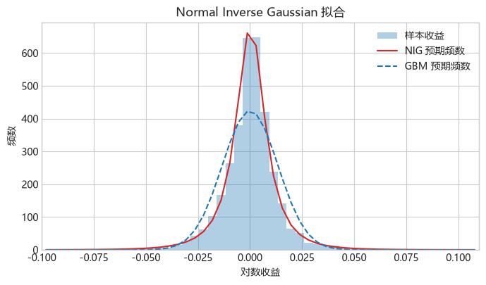

图 1.13 NIG 模型拟合的 2000 年 1 月至 2013 年 6 月 S&P 500 指数的对数收益，其中红色实线为拟合的 NIG 模型对应的每箱预期频数，而蓝色虚线为相应的GBM结果。整体图的模型频数通过各箱密度积分计算。

看起来NIG模型是本节中考虑的四个模型中拟合尾部和峰态效果最好的。

接着比较 NIG 模型与 GBM 在左右尾部的拟合。

# 图 1.13a：Normal Inverse Gaussian 与 GBM 在左尾的比较
nig_expected_counts = (
    nig_increment_density(
        tail_return_grid,
        nig_sigma,
        nig_nu,
        nig_theta,
        nig_c,
        time_step,
    )
    * len(log_returns)
    * tail_bin_width
)
plot_tail_comparison(
    tail_return_grid,
    tail_bin_centres,
    histogram_counts,
    tail_bin_width,
    gbm_expected_counts,
    nig_expected_counts,
    "Normal Inverse Gaussian",
    (log_returns.min(), -0.02),
    "Normal Inverse Gaussian 与 GBM：左尾",
)
plt.show()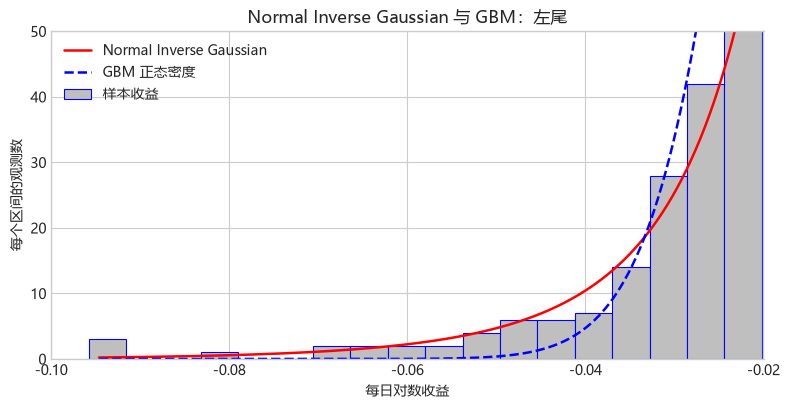

图 1.13a Normal Inverse Gaussian 模型与 GBM 在左尾的比较。

# 图 1.13b：Normal Inverse Gaussian 与 GBM 在右尾的比较
plot_tail_comparison(
    tail_return_grid,
    tail_bin_centres,
    histogram_counts,
    tail_bin_width,
    gbm_expected_counts,
    nig_expected_counts,
    "Normal Inverse Gaussian",
    (0.02, log_returns.max()),
    "Normal Inverse Gaussian 与 GBM：右尾",
)
plt.show()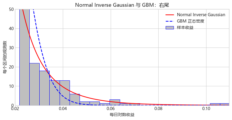

图 1.13b Normal Inverse Gaussian 模型与 GBM 在右尾的比较。

四种模型的样本内拟合比较

每个观测值的平均对数似然为 \(n^{-1}\sum_i\log f(x_i)\)，越大表示模型对这组已观测收益赋予的整体密度越高。分箱总变差为 \(\frac12\sum_j|\widehat p_j-p_j|\)，越小表示模型频率与样本频率越接近；计算时也包含绘图区间两端之外的概率。尾部概率使用 \(a\in\{3\%,4\%\}\) 两个日对数收益阈值：左尾概率为 \(P(X<-a)\)，右尾概率为 \(P(X>a)\)，可分别与相应的样本比例比较。

# 表 1.4：四种模型在同一历史样本上的定量比较
fitted_densities = {
    "GBM": lambda x: norm.pdf(x, loc=sample_mean, scale=np.sqrt(sample_variance)),
    "Merton": lambda x: merton_increment_density(
        x, merton_drift, merton_diffusion_volatility,
        merton_jump_intensity, 0.0, merton_jump_std, time_step),
    "VG": lambda x: variance_gamma_increment_density(
        x, vg_sigma, vg_nu, vg_theta, vg_c, time_step),
    "NIG": lambda x: nig_increment_density(
        x, nig_sigma, nig_nu, nig_theta, nig_c, time_step),
}
fitted_bin_counts = {
    "GBM": normal_bin_counts, "Merton": merton_bin_counts,
    "VG": vg_bin_counts, "NIG": nig_bin_counts,
}
observed_counts, _ = np.histogram(log_returns, bins=fit_bin_edges)
observed_probabilities = np.r_[
    np.mean(log_returns < fit_bin_edges[0]),
    observed_counts / len(log_returns),
    np.mean(log_returns > fit_bin_edges[-1]),
]
comparison_rows = []
for model_name, density in fitted_densities.items():
    left_outside = quad(density, -np.inf, fit_bin_edges[0])[0]
    right_outside = quad(density, fit_bin_edges[-1], np.inf)[0]
    probabilities = np.r_[left_outside,
                          fitted_bin_counts[model_name] / len(log_returns),
                          right_outside]
    comparison_rows.append({
        "模型": model_name,
        "平均对数似然（越大越好）": np.mean(np.log(density(log_returns))),
        "分箱总变差": 0.5 * np.sum(np.abs(observed_probabilities - probabilities)),
        "左尾概率（低于 -3%）": quad(density, -np.inf, -0.03)[0],
        "右尾概率（高于 3%）": quad(density, 0.03, np.inf)[0],
        "左尾概率（低于 -4%）": quad(density, -np.inf, -0.04)[0],
        "右尾概率（高于 4%）": quad(density, 0.04, np.inf)[0],
    })
fit_comparison = pd.DataFrame(comparison_rows).set_index("模型")
fit_comparison.loc["样本", :] = [np.nan, np.nan,
    np.mean(log_returns < -0.03), np.mean(log_returns > 0.03),
    np.mean(log_returns < -0.04), np.mean(log_returns > 0.04)]
fit_comparison

	平均对数似然（越大越好）	分箱总变差	左尾概率（低于 -3%）	右尾概率（高于 3%）	左尾概率（低于 -4%）	右尾概率（高于 4%）
模型
GBM	2.897977	0.165333	0.012196	0.012335	0.001348	0.001367
Merton	2.999307	0.100533	0.014816	0.014874	0.008601	0.008626
VG	2.958058	0.130640	0.024674	0.022531	0.011307	0.009952
NIG	3.022572	0.040682	0.021384	0.019559	0.009691	0.008496
样本	NaN	NaN	0.019458	0.018278	0.008550	0.007370

表 1.4 统一样本及分箱下的拟合指标。

比较结论。

• 整体拟合：NIG 最好，其次是 Merton、VG 和 GBM。 两项整体指标给出相同排序。NIG 的平均对数似然最高，为 3.0226，分箱总变差最小，为 0.0407；GBM 的对应值为 2.8980 和 0.1653。三种带跳跃的模型均改善了相对于 GBM 的整体拟合。
• GBM 低估了超过 \(\pm3\%\) 和 \(\pm4\%\) 的收益概率。 在 3% 阈值处，GBM 的左右尾概率为 1.22% 和 1.23%，样本比例为 1.95% 和 1.83%；在 4% 阈值处，GBM 的左右尾概率降至 0.135% 和 0.137%，样本比例仍为 0.855% 和 0.737%。这些结果量化了正态分布对极端收益概率的低估。
• NIG 在 3% 阈值处最接近样本的左右尾概率；在 4% 阈值处，Merton 最接近左尾，NIG 最接近右尾。 NIG 在 3% 阈值处的左右尾概率为 2.14% 和 1.96%。在 4% 阈值处，Merton 的左尾概率为 0.860%，接近样本的 0.855%；NIG 的右尾概率为 0.850%，接近样本的 0.737%。因此，NIG 的整体拟合最好，而 Merton 也能准确刻画本样本低于 -4% 的收益发生频率。

1.7 风险中性定价

1.7.1 风险中性世界

风险中性定价由 Cox 和 Ross（1976）提出。在风险中性世界中，任何资产的收益率都和无风险收益率相等，同时任何资产的定价都仅需要将未来现金流按照无风险利率贴现。比如，记风险中性世界为 \(Q\)，则股票价格在未来时刻 \(t>0\) 的在风险中性世界期望为

\[E^Q[S_t]=S_0e^{rt}.\]

如果标的资产 \(S\) 在风险中性世界中的动态已知，任何以 \(S\) 为标的资产的欧式期权都可以通过式（1.7.1）定价：

\[V_t(S)=e^{-r(T-t)}E^Q[V_T\mid S_t=S]\tag{1.7.1}.\]

这就是欧式期权的风险中性定价公式。

风险中性定价的依据是无套利与复制：对于可由股票和无风险资产交易复制的期权收益，期权价格等于复制组合的成本。第 4.1 节通过 Delta 对冲推导 Black–Scholes–Merton 偏微分方程，并由 Feynman–Kac 公式将其解写成式（1.7.1）的风险中性贴现期望。

风险中性定价的优点是把风险调整体现在 \(Q\) 下的概率分布中，而贴现统一使用无风险利率 \(r\)。给定风险中性模型后，定价只需计算未来收益的期望并贴现，无需另外估计标的资产在真实世界中的预期收益率，或为每一份期权设定风险调整贴现率。

例如，在无分红的 GBM 模型中，风险中性对数漂移为 \(r-\sigma^2/2\)，由无风险利率和波动率确定。因此，欧式期权价格可以根据当前股价、行权价、剩余期限、无风险利率和波动率计算。这也把后续数值方法的任务明确为：在给定的风险中性分布下计算期权收益的期望。

接下去分别调整四种对数收益过程的确定性漂移，使股票满足 \(E^Q[S_t]=S_0e^{rt}\)。

1.7.1.1 用矩生成函数确定风险中性漂移

先把对数价格写成

\[S_t=S_0e^{X_t},\quad X_t=c_Qt+Y_t,\]

其中 \(Y_t\) 是具有平稳独立增量的随机部分，\(c_Q\) 表示风险中性世界中指数内的确定性漂移。贴现后的股票价格必须满足

\[E^Q[e^{-rt}S_t]=S_0.\]

代入 \(S_t\) 并除以 \(S_0\)，得到

\[e^{-rt}e^{c_Qt}E^Q[e^{Y_t}]=1.\]

记 \(Y_t\) 的矩生成函数为 \(M_{Y_t}(u)=E^Q[e^{uY_t}]\)，其累积生成函数为 \(K_{Y_t}(u)=\log M_{Y_t}(u)\)。于是

\[e^{c_Qt}M_{Y_t}(1)=e^{rt},\quad c_Q=r-\frac{K_{Y_t}(1)}{t}.\]

这就是通过矩生成函数求风险中性漂移的通用公式：先求风险中性随机部分的 \(K_{Y_t}(1)\)，再从 \(r\) 中减去其单位时间贡献 \(K_{Y_t}(1)/t\)。

1.7.1.2 几何布朗运动

在风险中性世界中，记随机部分 \(Y_t=\sigma W_t\)。其矩生成函数和累积生成函数分别为

\[ M_{Y_t}(u)=E^Q[e^{uY_t}]=e^{\sigma^2u^2t/2}, \qquad K_{Y_t}(u)=\log M_{Y_t}(u)=\frac{1}{2}\sigma^2u^2t. \]

将 \(u=1\) 代入通用公式 \(c_Q=r-K_{Y_t}(1)/t\)，得到

\[ c_Q^{GBM}=r-\frac{1}{2}\sigma^2. \]

因此风险中性 GBM 为

\[ S_t=S_0\exp\left((r-\tfrac12\sigma^2)t+\sigma W_t\right), \quad W_t\sim N(0,t), \]

或者等价地，

\[ X_t\sim N\left((r-\sigma^2/2)t,\sigma^2t\right). \]

对到期日 \(T\)，也可写为

\[ S_T=S_0\exp\left((r-\tfrac12\sigma^2)T+\sigma\sqrt{T}Z\right), \quad Z\sim N(0,1). \]

1.7.1.3 Merton 跳跃扩散过程

在风险中性世界中，把随机部分记为 \(Y_t=\sigma W_t+\sum_{i=1}^{N_t}J_i\)，其中 \(N_t\sim\operatorname{Poisson}(\lambda t)\)，\(J_i\sim N(a,b^2)\)。给定 \(N_t=n\) 后，复合跳跃项的矩生成函数为

\[ E^Q\left[e^{u\sum_{i=1}^{N_t}J_i}\mid N_t=n\right] =\left(M_J(u)\right)^n, \qquad M_J(u)=E^Q[e^{uJ_1}]. \]

对 Poisson 跳跃次数取期望，得到

\[ \begin{aligned} E^Q\left[e^{u\sum_{i=1}^{N_t}J_i}\right] &=\sum_{n=0}^{\infty}\left(M_J(u)\right)^n \frac{e^{-\lambda t}(\lambda t)^n}{n!}\\ &=\exp\left(\lambda t\left[M_J(u)-1\right]\right). \end{aligned} \]

利用布朗部分与跳跃部分独立，随机部分的矩生成函数和累积生成函数为

\[ \begin{aligned} M_{Y_t}(u) &=\exp\left\{t\left(\frac{\sigma^2u^2}{2} +\lambda[M_J(u)-1]\right)\right\},\\ K_{Y_t}(u) &=\log M_{Y_t}(u) =t\left(\frac{\sigma^2u^2}{2} +\lambda[M_J(u)-1]\right). \end{aligned} \]

由于 \(J_1\sim N(a,b^2)\)，有

\[ M_J(u)=e^{au+b^2u^2/2}, \qquad M_J(1)=e^{a+b^2/2}. \]

由通用公式 \(c_Q=r-K_{Y_t}(1)/t\)，Merton 模型的总风险中性对数漂移为

\[ c_Q^{JD}=r-\frac{\sigma^2}{2} -\lambda\left(e^{a+b^2/2}-1\right). \]

把跳跃带来的额外修正记为 \(q_{JD}=-\lambda[M_J(1)-1]\)，便可写成

\[ q_{JD}=-\lambda\left(e^{a+b^2/2}-1\right), \qquad c_Q^{JD}=r-\frac{\sigma^2}{2}+q_{JD}. \]

1.7.1.4 指数 VG 过程

对指数 VG 过程，令 \(G_t=\gamma(t;1,\nu)\)，随机部分为

\[ Y_t=\theta G_t+\sigma W_{G_t}. \]

先固定业务时钟 \(G_t=g\)。此时 \(W_g\sim N(0,g)\)，并且 \(Y_t\mid G_t=g=\theta g+\sigma W_g\)。利用正态随机变量的矩生成函数 \(E[e^{sW_g}]=e^{s^2g/2}\)，得到

\[ \begin{aligned} E^Q[e^{uY_t}\mid G_t=g] &=e^{u\theta g}E^Q[e^{u\sigma W_g}]\\ &=e^{u\theta g+\sigma^2u^2g/2} =e^{v(u)g},\\ v(u)&=u\theta+\frac{1}{2}\sigma^2u^2. \end{aligned} \]

再对随机时钟取期望（全期望公式），便有

\[ M_{Y_t}(u)=E^Q[e^{uY_t}] =E^Q\!\left[E^Q[e^{uY_t}\mid G_t]\right] =E^Q[e^{v(u)G_t}]. \]

因此，\(Y_t\) 的矩生成函数就是 Gamma 时钟的矩生成函数在 \(v=v(u)\) 处的值。此处 \(G_t\sim\operatorname{Gamma}(k,\text{scale}=\nu)\)，其中 \(k=t/\nu\)，其密度为

\[ f_{G_t}(g)=\frac{g^{k-1}e^{-g/\nu}}{\nu^k\Gamma(k)},\quad g>0. \]

直接积分可得时钟的矩生成函数。对 \(v<1/\nu\)，令 \(a=1/\nu-v>0\)，并使用 Gamma 积分 \(\int_0^\infty g^{k-1}e^{-ag}\,dg=\Gamma(k)a^{-k}\)：

\[ \begin{aligned} E^Q[e^{vG_t}] &=\frac{1}{\nu^k\Gamma(k)} \int_0^\infty g^{k-1}e^{-(1/\nu-v)g}\,dg\\ &=\frac{\Gamma(k)(1/\nu-v)^{-k}} {\nu^k\Gamma(k)} =(1-\nu v)^{-k}. \end{aligned} \]

代入 \(k=t/\nu\) 及 \(v(u)=u\theta+\sigma^2u^2/2\)，得到 VG 随机部分的矩生成函数；取对数即为累积生成函数：

\[ \begin{aligned} M_{Y_t}(u) &=\left(1-\theta\nu u-\frac{\sigma^2\nu u^2}{2}\right)^{-t/\nu},\\ K_{Y_t}(u) &=\log M_{Y_t}(u) =-\frac{t}{\nu}\log\left(1-\theta\nu u -\frac{\sigma^2\nu u^2}{2}\right). \end{aligned} \]

由 \(c_Q=r-K_{Y_t}(1)/t\)，有

\[ q_{VG}=-\frac{K_{Y_t}(1)}{t} =\frac{1}{\nu}\log\left(1-\theta\nu-\frac{\sigma^2\nu}{2}\right), \qquad c_Q^{VG}=r+q_{VG}. \]

因此风险中性指数 VG 过程可写成

\[ S_t=S_0\exp\left((r+q_{VG})t+Y_t\right). \]

在 \(1-\theta\nu-\sigma^2\nu/2>0\) 的参数范围内，\(M_{Y_t}(1)\) 有限，代入上述补偿项后得到 \(E^Q[S_t]=S_0e^{rt}\)。

1.7.1.5 指数 NIG 过程

对指数 NIG 过程，令 \(G_t=IG(t;1,1/\nu)\)，随机部分为

\[ Y_t=\theta G_t+\sigma W_{G_t}. \]

VG 与 NIG 的条件正态部分相同。给定 \(G_t=g\)，有 \(Y_t\mid G_t=g\sim N(\theta g,\sigma^2g)\)，所以令

\[ v(u)=u\theta+\frac{1}{2}\sigma^2u^2, \qquad M_{Y_t}(u)=E^Q[e^{v(u)G_t}]. \]

区别在于 NIG 的业务时钟为逆高斯分布。在本章的参数化下，\(G_t\) 的均值为 \(t\)、方差为 \(\nu t\)，其密度为

\[ f_{G_t}(g)=\frac{t}{\sqrt{2\pi\nu g^3}} \exp\left(-\frac{(g-t)^2}{2\nu g}\right),\quad g>0. \]

将密度代入时钟的矩生成函数，并整理指数项：

\[ \begin{aligned} E^Q[e^{vG_t}] &=\frac{t e^{t/\nu}}{\sqrt{2\pi\nu}} \int_0^\infty g^{-3/2} \exp\left[-\frac{1-2\nu v}{2\nu}g -\frac{t^2}{2\nu g}\right]dg. \end{aligned} \]

使用积分恒等式

\[ \int_0^\infty g^{-3/2}e^{-Ag-B/g}\,dg =\sqrt{\frac{\pi}{B}}e^{-2\sqrt{AB}},\quad A,B>0, \]

其中 \(A=(1-2\nu v)/(2\nu)\)、\(B=t^2/(2\nu)\)。整理后得到逆高斯时钟的矩生成函数

\[ E^Q[e^{vG_t}] =\exp\left[\frac{t}{\nu} \left(1-\sqrt{1-2\nu v}\right)\right], \quad v<\frac{1}{2\nu}. \]

在边界 \(v=1/(2\nu)\) 上，积分中的 \(A=0\)；此时积分仍收敛，MGF 等于 \(e^{t/\nu}\)。因此上式可连续延伸到这个边界。

将 \(v(u)=u\theta+\sigma^2u^2/2\) 代回 \(M_{Y_t}(u)=E^Q[e^{v(u)G_t}]\)，再取对数，得到 NIG 随机部分的矩生成函数和累积生成函数：

\[ \begin{aligned} M_{Y_t}(u) &=\exp\left\{\frac{t}{\nu} \left(1-\sqrt{1-2\theta\nu u-\sigma^2\nu u^2}\right)\right\},\\ K_{Y_t}(u) &=\log M_{Y_t}(u) =\frac{t}{\nu} \left(1-\sqrt{1-2\theta\nu u-\sigma^2\nu u^2}\right). \end{aligned} \]

由 \(c_Q=r-K_{Y_t}(1)/t\)，得到

\[ q_{NIG}=-\frac{K_{Y_t}(1)}{t} =-\frac{1}{\nu}\left(1-\sqrt{1-2\theta\nu-\sigma^2\nu}\right), \qquad c_Q^{NIG}=r+q_{NIG}. \]

NIG 的 MGF 在根号内非负时有限，因此 \(u=1\) 的条件为 \(1-2\theta\nu-\sigma^2\nu\geq0\)。边界上 \(M_{Y_t}(1)=e^{t/\nu}\)。对 MGF 求导会产生 \((1-2\theta\nu u-\sigma^2\nu u^2)^{-1/2}\) 因子，因此求导所用的参数范围取根号内严格为正。

对于 VG 和 NIG，补偿项都满足 \(q=-K_{Y_t}(1)/t\)，所以

\[ e^{-qt}=E^Q[e^{Y_t}]=M_{Y_t}(1)=e^{K_{Y_t}(1)}. \]

这与通用公式 \(c_Q=r-K_{Y_t}(1)/t\) 相同；矩生成函数和累积生成函数的定义及性质将在第 5 章进一步介绍。

本节符号 \(q\) 表示对数价格过程的风险中性补偿项。历史拟合中的 \(c\) 由样本均值确定：\(\hat c=\bar x/h-\hat\theta\)；风险中性漂移则由 \(c_Q=r-K_{Y_t}(1)/t\) 确定。前者匹配历史收益的均值，后者匹配股票的风险中性期望增长率。

综上所述，表 1.3 给出了各种随机过程在风险中性世界中的漂移率。

分布	参数	风险中性世界对数漂移率
布朗运动	\((\mu,\sigma)\)	\(r-\sigma^2/2\)
Merton 跳跃扩散	\((\mu,\sigma,\lambda,a,b)\)	\(r-\sigma^2/2-\lambda(e^{a+b^2/2}-1)\)
VG	\((\theta,\sigma,\nu)\)	\(r+\nu^{-1}\log(1-\theta\nu-\sigma^2\nu/2)\)
NIG	\((\theta,\sigma,\nu)\)	\(r-\nu^{-1}(1-\sqrt{1-2\theta\nu-\sigma^2\nu})\)

表 1.3 各种随机过程在风险中性世界中的漂移率

1.8 Black–Scholes 公式

Black–Scholes–Merton（BSM）模型是假设股票价格服从几何布朗运动的模型。期权价格由以下因素决定：

• 标的资产当前价格 \(S_0\)；
• 标的资产波动率 \(\sigma\)；
• 期权行权价 \(K\)；
• 期权期限 \(T\)；
• 无风险利率 \(r\)。

基于以下额外的假设：

1. 市场存在无风险利率，投资者可以按无风险利率存钱和借钱；
2. 标的资产不支付股息；
3. 交易成本为零，没有买卖价差；
4. 股票可分割，可以持有或卖空任意数量的股票。

Black 和 Scholes（1973）给出了欧式股票期权价格的解析表达式，被命名为 Black–Scholes 公式；这是最广泛应用的期权定价公式。

根据风险中性定价原理，在定价到期日为 \(T\)、标的为 \(S\) 的期权时，若 \(S_T=S_0e^{X_T}\) 服从几何布朗运动，那么

\[ X_T\sim N\left((r-\sigma^2/2)T,\sigma^2T\right). \]

对看涨期权，先计算到期收益的期望：

\[ \begin{aligned} E^Q[(S_T-K)^+] &=E^Q[(S_0e^{X_T}-K)^+]\\ &=\int_{\log(K/S_0)}^{+\infty}(S_0e^x-K) \frac{1}{\sqrt{2\pi\sigma^2T}} \exp\left[-\frac{(x-(r-\sigma^2/2)T)^2}{2\sigma^2T}\right]dx. \end{aligned} \]

把 \([x-(r-\sigma^2/2)T]/(\sigma\sqrt T)\) 替换为 \(y\)，令

\[ y=\frac{x-(r-\sigma^2/2)T}{\sigma\sqrt T},\quad a=\frac{\log(K/S_0)-(r-\sigma^2/2)T}{\sigma\sqrt T}=-d_2. \]

把 \([x-(r-\sigma^2/2)T]/(\sigma\sqrt T)\) 替换为 \(y\) 后，得到

\[ \begin{aligned} E^Q[(S_T-K)^+] =&\int_a^{+\infty} \left(S_0e^{\sigma\sqrt T y+(r-\sigma^2/2)T}-K\right)\phi(y)\,dy\\ =&S_0e^{rT}\int_a^{+\infty} e^{\sigma\sqrt T y-\sigma^2T/2}\phi(y)\,dy -K\int_a^{+\infty}\phi(y)\,dy. \end{aligned} \]

显然上式中第二项的积分是标准正态分布的尾概率；第一项在使用替换 \(z=y-\sigma\sqrt T\) 后也成为标准正态分布的尾概率。对标准正态密度 \(\phi\)，第二项可以写为

\[ K\Phi\left(\frac{\log(S_0/K)+(r-\sigma^2/2)T} {\sigma\sqrt T}\right). \]

其中 \(\Phi\) 表示标准正态分布函数。而第一项在使用替换 \(z=y-\sigma\sqrt T\) 后也成为标准正态分布的尾概率，从而第一项可以写为

\[ S_0e^{rT}\Phi\left(\frac{\log(S_0/K)+(r+\sigma^2/2)T} {\sigma\sqrt T}\right). \]

因为欧式看涨期权在 \(t\) 的价格是 \(C(S,t)=e^{-r(T-t)}E^Q[(S_T-K)^+\mid S_t=S]\)，根据以上推导 \(C(S,t)\) 可以由以下公式给出

\[ C(S,t)=S\Phi(d_1)-Ke^{-r(T-t)}\Phi(d_2) \tag{1.8.1} \]

其中

\[ d_1=\frac{\log(S/K)+(r+\sigma^2/2)(T-t)} {\sigma\sqrt{T-t}} \tag{1.8.2} \]

\[ d_2=d_1-\sigma\sqrt{T-t} \tag{1.8.3} \]

看涨期权公式的两项也有直观含义。在无分红 BSM 模型下，\(\Phi(d_2)\) 是风险中性世界中到期股价超过执行价的概率，因此 \(Ke^{-r(T-t)}\Phi(d_2)\) 对应需要支付的执行价的期望现值；\(S\Phi(d_1)\) 对应取得股票部分的期望现值。\(d_2\) 来自行权条件 \(S_T>K\) 的门槛，而计算股票部分的期望时，每个行权情景还要按到期股价 \(S_T\) 加权：股价越高，对这一项的贡献越大。这一步加权使正态分布函数的参数变为 \(d_1=d_2+\sigma\sqrt{T-t}\)，因此定价公式包含两个不同的正态分布函数值。

这就是著名的 Black–Scholes 公式。看跌期权可以用同样的方法得到欧式看跌期权的价格。当然，看跌期权的价格也可以通过买权卖权平价关系得到。

1.8.1 买权卖权平价关系

让我们用 \(\omega\) 代表欧式期权在 \(T\) 可能实现的任意情景。根据看涨期权和看跌期权的定义，它们在该情景下的贴现到期收益分别为

\[ \widetilde g_C(\omega)=e^{-rT}(S_T(\omega)-K)^+, \quad \widetilde g_P(\omega)=e^{-rT}(K-S_T(\omega))^+. \]

不管是 \(S_T(\omega)\geq K\)，还是 \(S_T(\omega)<K\)，不难验证以下等式都成立：

\[ \widetilde g_C(\omega)-\widetilde g_P(\omega)=e^{-rT}(S_T(\omega)-K). \]

对其两边取期望，我们可以得到所谓的买权卖权平价关系，

\[ C-P=e^{-rT}E^Q[S_T-K]=S_0-e^{-rT}K \tag{1.8.4} \]

买权卖权平价关系的到期收益比较

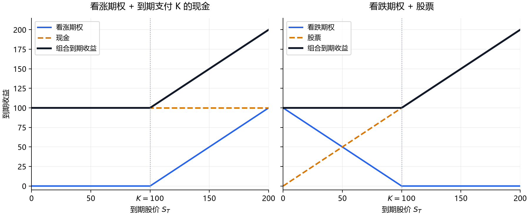
买权卖权平价关系示意图（\(K=100\)）。左图为看涨期权与到期支付 \(K\) 的现金组合，右图为看跌期权与股票组合。两者的到期收益均为 \(\max(S_T,K)\)，因此当前成本满足 \(C+Ke^{-rT}=P+S_0\)。

在 BSM 模型中，我们可以套入看涨期权的定价公式（1.8.1）得到

\[ \begin{aligned} P(S,t)&=C(S,t)+Ke^{-r(T-t)}-S\\ &=Ke^{-r(T-t)}\Phi(-d_2)-S\Phi(-d_1) \end{aligned} \tag{1.8.5} \]

上述看涨和看跌欧式期权价格可以由 Python 程序 1.10 计算。

# 参数定义：固定的 BSM 示例参数
S0 = 100.0
K = 100.0
T = 1.0
r = 0.05
sigma = 0.20

公式与代码对应

d1、d2 对应定价公式中的 \(d_1,d_2\)；T 表示剩余到期时间。discount 对应 \(e^{-rT}\)，norm.cdf 用于计算标准正态分布函数 \(\Phi\)。

Python程序 1.10：Black–Scholes 中间量函数与看涨、看跌期权统一定价函数（cp=1 表示看涨，cp=-1 表示看跌）

def black_scholes_d1_d2(sigma, S0, K, T, r):
    """Return the two standardized distances used in the BSM formula."""
    d1 = (np.log(S0 / K) + (r + sigma**2 / 2) * T) / (sigma * np.sqrt(T))
    d2 = d1 - sigma * np.sqrt(T)
    return d1, d2


def black_scholes_formula(sigma, S0, K, T, r, cp):
    """Return a no-dividend European call (cp=1) or put (cp=-1) value."""
    if cp not in (-1, 1):
        raise ValueError("cp must be 1 for a call or -1 for a put")
    d1, d2 = black_scholes_d1_d2(sigma, S0, K, T, r)
    discount = np.exp(-r * T)
    return cp * (S0 * norm.cdf(cp * d1) - K * discount * norm.cdf(cp * d2))


# 接口前五个参数沿用 def black_scholes_formula(sigma, S0, K, T, r) 的顺序，cp 是第六个参数。

# 用模型对象和期权对象组织程序 1.10 的输入
from quant_option_pricing import BlackScholesModel, EuropeanOption

model = BlackScholesModel(rate=r, volatility=sigma)
call_option = EuropeanOption.call(spot=S0, strike=K, maturity=T)
put_option = EuropeanOption.put(spot=S0, strike=K, maturity=T)

d1, d2 = black_scholes_d1_d2(
    model.volatility,
    call_option.spot,
    call_option.strike,
    call_option.maturity,
    model.rate,
)
call_value = black_scholes_formula(
    model.volatility,
    call_option.spot,
    call_option.strike,
    call_option.maturity,
    model.rate,
    call_option.cp,
)
put_value = black_scholes_formula(
    model.volatility,
    put_option.spot,
    put_option.strike,
    put_option.maturity,
    model.rate,
    put_option.cp,
)
pd.Series({"d1": d1, "d2": d2, "看涨期权": call_value, "看跌期权": put_value})

d1       0.350000
d2       0.150000
看涨期权    10.450584
看跌期权     5.573526
dtype: float64

1.9 敏感性参数

期权的敏感性参数(sensitivity,也被称为Greeks)是指期权价格对于相关变量或者参数发生变化的敏感性。这些敏感性参数作为期权的风险指标，可以用于期权风险的控制和管理。

1.9.1 Delta

最重要的敏感性参数是 Delta。Delta 衡量标的资产价格变动时，期权价格的变化幅度，即

\[ \Delta=\frac{\partial V}{\partial S} \tag{1.9.1} \]

暂时忽略时间这一维度，将期权价格 \(V\) 在股票当前价格 \(S_0\) 处展开为泰勒级数(Taylor series)可以得到

\[ V(S) \approx V(S_0) + \dfrac{\partial V}{\partial S}(S-S_0) +\dfrac{1}{2}\dfrac{\partial^2 V}{\partial S^2}(S-S_0)^2 \tag{1.9.2} \]

若标的资产价格仅发生细微变化，则二阶导数项可以忽略不计，式（1.9.2）可以简化为

\[ V(S) - V(S_0) = \Delta(S-S_0). \]

持有 1 份期权和 \(-\Delta\) 股标的资产，组合的一阶股价敏感度为 \(\Delta-\Delta=0\)，那么该投资组合的价值将保持恒定为

\[ V(S)-\Delta S = V(S_0)-\Delta S_0. \]

该组合因此被称为是 Delta 中性组合(Delta neutral portfolio)。

然而由于 Delta 是资产价格的函数，所以当资产价格发生变化时，Delta 也会变化。此时要想保持投资组合的 Delta 中性，必须调整投资组合期权与股票的比例与新的 Delta 一致。

1.9.2 Gamma

期权的另一敏感性参数 Gamma 反映了标的资产价格对 Delta 值的影响程度，

\[ \Gamma = \dfrac{\partial \Delta}{\partial S} = \dfrac{\partial^2 V}{\partial S^2} \tag{1.9.3} \]

当股价小幅变化 \(\delta S\) 时，Delta 的变化约为 \(\Gamma\,\delta S\)。若持有一份期权，并用 \(-\Delta\) 股股票对冲，为恢复 Delta 中性，股票仓位需调整约 \(-\Gamma\,\delta S\) 股。因此，对于相同的股价变动，Gamma 的绝对值越大，需要调整的对冲仓位越多。

同时我们也指出，期权价格的泰勒展开式可以改写为

\[ V(S)-V(S_0)\approx \Delta(S-S_0)+\dfrac{1}{2}\Gamma(S-S_0)^2. \tag{1.9.4} \]

这一估计提供了当标的资产价格发生变化时期权价格的变化，被称为期权价格的 Delta-Gamma 估计。该估计是价值函数 \(V(S)\) 在 \(S_0\) 处的二阶泰勒展开，可用于正态及前面介绍的尖峰厚尾收益模型产生的价格情景。若股票仓位保持为 \(-\Delta\)，组合的一阶变化相互抵消，二阶价值变化约为 \(\tfrac12\Gamma(S-S_0)^2\)。

1.9.3 Theta

Theta 用于测量时间变化对期权理论价值的影响。

\[ \Theta = \dfrac{\partial V_t}{\partial t} \tag{1.9.5} \]

Theta 表示在标的价格及其他参数不变时，日历时间流逝对期权价格的局部影响。时间以年为单位，一个交易日取 \(h=1/250\)。经过这一时间间隔后，价格变化约为 \(\Theta h\)；负的 Theta 对应价值下降，正的 Theta 对应价值上升。

在式（1.9.4）的基础上加上 Theta 项，我们可以得到期权价格的 Delta-Gamma-Theta 估计。

\[ V(S,t)-V(S_0,t_0)\approx \Theta(t-t_0)+\Delta(S-S_0) +\dfrac{1}{2}\Gamma(S-S_0)^2. \tag{1.9.6} \]

1.9.4 Vega

Vega 衡量标的资产价格波动率变动时，期权价格的变化幅度，

\[ \nu = \dfrac{\partial V}{\partial \sigma}. \tag{1.9.7} \]

欧式看跌期权和看涨期权的 Vega 总是相等的。基于买权卖权平价关系 \(C-P=S_0-Ke^{-rT}=S_0-e^{-rT}K\)，对等式两边对波动率取偏导可以得到

\[ \dfrac{\partial}{\partial \sigma}(C-P)=\nu_C-\nu_P \tag{1.9.8} \]

\[ \dfrac{\partial}{\partial \sigma}(S_0-e^{-rT}K)=0. \tag{1.9.9} \]

所以 \(\nu_C-\nu_P=0\)，也就是 \(\nu_C=\nu_P\)。这里用 Vega 表示该敏感性参数，以免与 VG 和 NIG 模型中的时间变化参数 \(\nu\) 混淆。看涨和看跌期权的 Vega 相等且为正。

1.9.5 Rho

Rho 是指期权价格对无风险利率变化的敏感程度，

\[ \rho=\dfrac{\partial V_t}{\partial r} \tag{1.9.10} \]

利率变化 \(\delta r\) 带来的价格变化约为 \(\rho\,\delta r\)。下面的无分红 BSM 公式给出 \(|\rho|\leq K\tau e^{-r\tau}\)，其中 \(\tau=T-t\)；剩余期限缩短时，这一利率敏感度上界按 \(\tau\) 趋于零。例如，Rho 为 20 时，利率上升一个百分点，对应的价格变化约为 \(20\times0.01=0.20\)。

1.9.6 BSM 模型中的敏感性参数

我们首先给出 BSM 模型中看涨期权各种敏感性参数的表达式。

\[ \Delta_C=\Phi(d_1) \tag{1.9.11} \]

\[ \Gamma_C=\dfrac{\phi(d_1)}{S\sigma\sqrt{T-t}} \tag{1.9.12} \]

\[ \nu_C=S\phi(d_1)\sqrt{T-t} =Ke^{-r(T-t)}\phi(d_2)\sqrt{T-t} \tag{1.9.13} \]

\[ \Theta_C=-\dfrac{S\phi(d_1)\sigma}{2\sqrt{T-t}} -rKe^{-r(T-t)}\Phi(d_2) \tag{1.9.14} \]

\[ \rho_C=K(T-t)e^{-r(T-t)}\Phi(d_2) \tag{1.9.15} \]

在 \(S,K,\sigma,T-t>0\) 且 \(r\geq0\) 的无分红 BSM 模型中，看涨期权的 Delta、Gamma、Vega 和 Rho 为正，Theta 为负。

而看跌期权各种敏感性参数为

\[ \Delta_P=-\Phi(-d_1)=\Delta_C-1 \tag{1.9.16} \]

\[ \Gamma_P=\Gamma_C \tag{1.9.17} \]

\[ \nu_P=\nu_C \tag{1.9.18} \]

\[ \Theta_P=-\dfrac{S\phi(-d_1)\sigma}{2\sqrt{T-t}} +rKe^{-r(T-t)}\Phi(-d_2)=\Theta_C+rKe^{-r(T-t)} \tag{1.9.19} \]

\[ \rho_P=-K(T-t)e^{-r(T-t)}\Phi(-d_2) \tag{1.9.20} \]

接下来我们演示如何推导看涨期权的 Delta、Gamma 和 Vega。推导过程需要用到以下两个有用的等式

\[ \dfrac{\partial \Phi(d_1)}{\partial d_1}=\phi(d_1) \tag{1.9.21} \]

\[ \dfrac{\partial \Phi(d_2)}{\partial d_2}=\phi(d_2) =\phi(d_1)e^{d_1\sigma\sqrt{T-t}}e^{-\frac{\sigma^2(T-t)}{2}} =\phi(d_1)S_te^{r(T-t)}/K. \tag{1.9.22} \]

将式（1.8.1）对 \(S_t\) 求导可以得到

\[ \begin{aligned} \Delta_C&=\Phi(d_1)+S_t\dfrac{\partial \Phi(d_1)}{\partial S_t} -Ke^{-r(T-t)}\dfrac{\partial \Phi(d_2)}{\partial S_t}\\ &=\Phi(d_1)+S_t\dfrac{\partial \Phi(d_1)}{\partial d_1} \dfrac{\partial d_1}{\partial S_t} -Ke^{-r(T-t)}\dfrac{\partial \Phi(d_2)}{\partial d_2} \dfrac{\partial d_2}{\partial S_t}\\ &=\Phi(d_1)+S_t\phi(d_1)\dfrac{1}{S_t\sigma\sqrt{T-t}} -Ke^{-r(T-t)}\phi(d_1)\dfrac{S_te^{r(T-t)}}{K} \dfrac{1}{S_t\sigma\sqrt{T-t}}\\ &=\Phi(d_1). \end{aligned} \]

其中 \(\partial d_1/\partial S_t=\partial d_2/\partial S_t=1/(S_t\sigma\sqrt{T-t})\)，并使用了式（1.9.22）。

将 Delta 对 \(S_t\) 求导可以得到

\[ \Gamma_C=\dfrac{\partial \Delta_C}{\partial S_t} =\dfrac{\partial \Phi(d_1)}{\partial d_1} \dfrac{\partial d_1}{\partial S_t} =\dfrac{\phi(d_1)}{S_t\sigma\sqrt{T-t}}. \]

而将式（1.8.1）对 \(\sigma\) 求导可以得到

\[ \begin{aligned} \nu_C&=S_t\dfrac{\partial \Phi(d_1)}{\partial \sigma} -Ke^{-r(T-t)}\dfrac{\partial \Phi(d_2)}{\partial \sigma}\\ &=S_t\dfrac{\partial \Phi(d_1)}{\partial d_1} \dfrac{\partial d_1}{\partial \sigma} -Ke^{-r(T-t)}\dfrac{\partial \Phi(d_2)}{\partial d_2} \dfrac{\partial d_2}{\partial \sigma}. \end{aligned} \]

将 \(d_1\) 和 \(d_2\) 分别对 \(\sigma\) 求导可以得到

\[ \begin{aligned} \dfrac{\partial d_1}{\partial \sigma} &=\dfrac{\sigma^2(T-t)^{3/2} -\left[\log\left(S/K\right)+\left(r+\sigma^2/2\right)(T-t)\right]\sqrt{T-t}} {\sigma^2(T-t)}\\ \dfrac{\partial d_2}{\partial \sigma} &=\dfrac{-\left[\log\left(S/K\right)+\left(r+\sigma^2/2\right)(T-t)\right]\sqrt{T-t}} {\sigma^2(T-t)}. \end{aligned} \]

因此

\[ \nu_C=S\phi(d_1)\sqrt{T-t} =Ke^{-r(T-t)}\phi(d_2)\sqrt{T-t}. \tag{1.9.23} \]

使用 Greeks 时要同时注意变化的单位和近似范围。若股价变化 \(\delta S\)，Delta 给出的价格变化约为 \(\Delta\,\delta S\)；加入 Gamma 后，再计入 \(\tfrac12\Gamma(\delta S)^2\)。Delta 中性组合抵消当前位置附近的一阶股价影响；股价移动后，Gamma 带来二阶价格变化，Delta 也随之改变，因此需要重新调整持仓。Vega 按波动率的小数值计量，“上升一个百分点”对应波动率增加 0.01：例如 Vega 为 20 时，从 20% 升到 21% 的价格变化约为 \(20\times0.01=0.20\)。取时间步长 \(h=1/250\) 时，时间变化带来的价格变化约为 \(\Theta h\)。式（1.9.6）中的 Delta、Gamma 和 Theta 均取初始点 \((S_0,t_0)\) 的值，保留股价变化的一、二阶项和时间变化的一阶项。

公式与代码对应

density 对应标准正态密度 \(\phi(d_1)\)，discount 对应 \(e^{-rT}\)。返回字典中的 delta、gamma、vega、theta 和 rho 分别保存相应敏感性参数。

Python程序 1.11：Black–Scholes看涨期权Greeks函数、Black–Scholes看跌期权Greeks函数

def call_greeks_formula(sigma, S0, K, T, r):
    '''Return Delta, Gamma, Vega, Theta, and Rho for a call.'''
    d1 = (np.log(S0 / K) + (r + sigma**2 / 2) * T) / (sigma * np.sqrt(T))
    d2 = d1 - sigma * np.sqrt(T)
    density = norm.pdf(d1)
    discount = np.exp(-r * T)
    return {
        "delta": norm.cdf(d1),
        "gamma": density / (S0 * sigma * np.sqrt(T)),
        "vega": S0 * density * np.sqrt(T),
        "theta": -S0 * density * sigma / (2 * np.sqrt(T))
        - r * K * discount * norm.cdf(d2),
        "rho": K * T * discount * norm.cdf(d2),
    }

def put_greeks_formula(sigma, S0, K, T, r):
    '''Return Delta, Gamma, Vega, Theta, and Rho for a put.'''
    d1 = (np.log(S0 / K) + (r + sigma**2 / 2) * T) / (sigma * np.sqrt(T))
    d2 = d1 - sigma * np.sqrt(T)
    density = norm.pdf(d1)
    discount = np.exp(-r * T)
    return {
        "delta": norm.cdf(d1) - 1.0,
        "gamma": density / (S0 * sigma * np.sqrt(T)),
        "vega": S0 * density * np.sqrt(T),
        "theta": -S0 * density * sigma / (2 * np.sqrt(T))
        + r * K * discount * norm.cdf(-d2),
        "rho": -K * T * discount * norm.cdf(-d2),
    }

# 调用程序 1.11 计算看涨和看跌期权的 Greeks
call_greeks = call_greeks_formula(sigma, S0, K, T, r)
put_greeks = put_greeks_formula(sigma, S0, K, T, r)
pd.DataFrame({"看涨": call_greeks, "看跌": put_greeks})

	看涨	看跌
delta	0.636831	-0.363169
gamma	0.018762	0.018762
vega	37.524035	37.524035
theta	-6.414028	-1.657880
rho	53.232482	-41.890461

图 1.14 展示了 BSM 模型中，对应当前股价 \(0<S_0\leq 40\) 时，到期日为 \(T=0.1\) 年和 \(T=1\) 年的欧式看涨和看跌期权的价格，\(Delta\)，\(Gamma\)，\(Vega\) 和 \(Theta\)。该期权的其他参数为 \(\sigma=0.2\)，\(K=20\)，\(r=5\%\)。以下用 \(S\) 表示当前股价，用 \(\tau=T-t\) 表示剩余期限；图中 \(t=0\)，因此 \(\tau=T\)。根据图形我们总结以下 BSM 模型中敏感性参数的性质：

• 欧式看涨期权的 Delta 在 \((0,1)\) 之间，而欧式看跌期权的 Delta 在 \((-1,0)\) 之间。标的资产价格越高，Delta 越高。
• 欧式看涨和看跌期权的 Gamma 相等且为正。由式（1.9.12）对 \(S\) 求导，Gamma 的峰值满足 \(d_1=-\sigma\sqrt\tau\)，对应股价 \(S_\Gamma^*=K\exp[-(r+3\sigma^2/2)\tau]\)；股价向峰值两侧移动时 Gamma 下降。保持 \(K,r,\sigma\) 不变并令剩余期限 \(\tau\to0\)：在平值点 \(S=K\)，Gamma 约为 \(1/(K\sigma\sqrt{2\pi\tau})\)，随期限缩短而上升；若股价固定在某个 \(S<K\) 或 \(S>K\) 的位置，Gamma 则趋于零。临近到期时，期权价格曲线在执行价两侧逐渐接近直线，曲率集中在 \(K\) 附近越来越窄的区域，因此 Gamma 曲线的峰值升高，而远离执行价处的 Gamma 下降。
• 欧式看涨和看跌期权的 Vega 相等且为正。由式（1.9.13）对 \(S\) 求导，峰值满足 \(d_1=\sigma\sqrt\tau\)，对应股价 \(S_{\mathrm{Vega}}^*=K\exp[(\sigma^2/2-r)\tau]\)；股价向峰值两侧移动时 Vega 下降。保持 \(K,r,\sigma\) 不变并令 \(\tau\to0\) 时，Vega 对任何固定股价 \(S>0\) 都趋于零，包括平值点 \(S=K\)。平值 Vega 约为 \(K\sqrt{\tau/(2\pi)}\)，随剩余期限的平方根下降。剩余时间越短，波动率变化对到期股价分布的影响越小；到期时，收益由股价和执行价直接确定。因此，与 Gamma 的峰值升高不同，Vega 的峰值随临近到期而降低。
• 在无分红且 \(r\geq0\) 时，欧式看涨期权的 Theta 为负。看跌 Theta 为扩散项 \(-S\sigma\phi(d_1)/(2\sqrt\tau)\) 与利息项 \(rKe^{-r\tau}\Phi(-d_2)\) 之和；\(S\to0\) 且 \(r>0\) 时，前者趋于零，Theta 趋于 \(rKe^{-r\tau}>0\)。临近到期，平值看涨和看跌的 Theta 主导项均为 \(-K\sigma/(2\sqrt{2\pi\tau})\)，时间价值损失加速；当 \(\tau\to0\) 且股价固定时，看涨 Theta 在 \(S>K\) 时趋于 \(-rK\)，在 \(S<K\) 时趋于零；看跌 Theta 在 \(S<K\) 时趋于 \(rK\)，在 \(S>K\) 时趋于零。

Black–Scholes 模型中欧式看涨和看跌期权的价格及希腊字母。

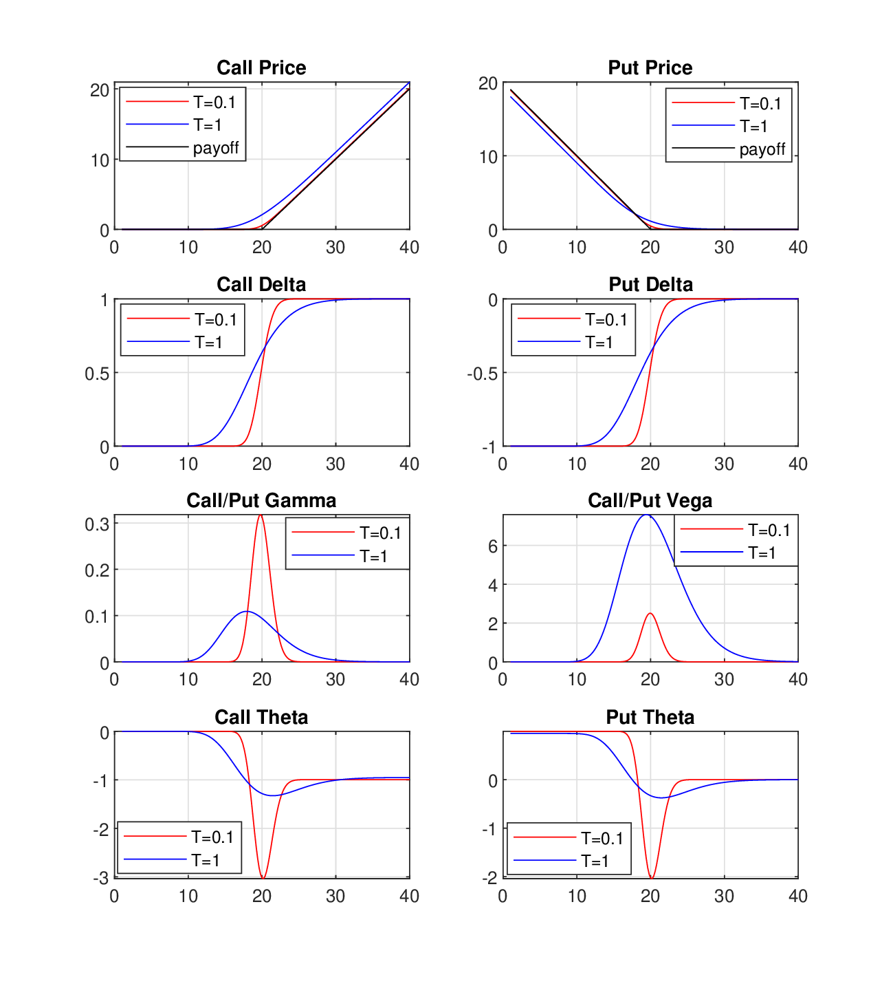
图 1.14 Black–Scholes 模型中欧式看涨和看跌期权的价格及希腊字母，其中 \(0<S_0\leq40\)、\(T\in\{0.1,1\}\)、\(\sigma=0.2\)、\(K=20\)、\(r=5\%\)。

1.9.7 BSM模型下的Delta-Gamma-Theta估计

之前我们已经介绍过期权价格的 Delta-Gamma-Theta 估计

\[ V(S,t)-V(S_0,t_0)\approx \Theta(t-t_0)+\Delta(S-S_0) +\dfrac{1}{2}\Gamma(S-S_0)^2. \tag{1.9.24} \]

作为一个期权价格估计方法，Delta-Gamma-Theta 被广泛应用于带有期权或其他金融衍生证券的投资组合的风险测量和管理。在交易组合的风险管理中，常需要估计未来一个风险期限内的组合损益分布，例如用于计算风险价值（Value at Risk）。获取投资组合价值的分布函数通常需要使用蒙特卡罗(Monte Carlo)产生大量资产价格 \(S\) 的场景，并在每一场景对期权重新定价。如果期权价格无法由解析式得到，而 Delta、Gamma 和 Theta 却已知，使用这一估计避免了在每一个情境下使用数值方法对期权重新定价的需要，可以节省大量时间。各情景共用初始点的 Delta、Gamma 和 Theta，只需计算式（1.9.24）中的三个项。

下面我们通过一个例子演示在 Black-Scholes 模型下 Delta-Gamma-Theta 估计的表现。首先计算 Black-Scholes 模型下的 Delta、Gamma 和 Theta。然后针对一系列不超过 \(\pm10\%\) 的 \(S\) 的日收益，使用 Black-Scholes 公式对期权重新定价，同时也通过 Delta-Gamma-Theta 来估计期权价格。

# 图 1.15：设置期权参数并计算初始价格和 Greeks
dgt_spot = 100.0
dgt_strike = 120.0
dgt_maturity = 1.0
dgt_rate = 0.05
dgt_volatility = 0.20
dgt_greeks = call_greeks_formula(
    dgt_volatility, dgt_spot, dgt_strike, dgt_maturity, dgt_rate
)
dgt_initial_value = black_scholes_formula(
    dgt_volatility, dgt_spot, dgt_strike, dgt_maturity, dgt_rate, cp=1
)
dgt_greeks

{'delta': np.float64(0.28719163790512714),
 'gamma': np.float64(0.017036921138505086),
 'vega': np.float64(34.07384227701017),
 'theta': np.float64(-4.680968546398613),
 'rho': np.float64(25.4716863739519)}

# 图 1.15：计算精确定价变化和 Delta–Gamma–Theta 近似
dgt_time_step = 1.0 / 250.0
dgt_price_changes = dgt_spot * np.arange(-0.10, 0.101, 0.01)
dgt_exact_changes = np.array(
    [
        black_scholes_formula(
            dgt_volatility,
            dgt_spot + price_change,
            dgt_strike,
            dgt_maturity - dgt_time_step,
            dgt_rate,
            1,
        )
        - dgt_initial_value
        for price_change in dgt_price_changes
    ]
)
approx_change = (
    dgt_greeks["theta"] * dgt_time_step
    + dgt_greeks["delta"] * dgt_price_changes
    + 0.5 * dgt_greeks["gamma"] * dgt_price_changes**2
)
pd.DataFrame(
    {
        "标的价格变化": dgt_price_changes,
        "精确变化": dgt_exact_changes,
        "Delta-Gamma-Theta 近似": approx_change,
    }
).head()

	标的价格变化	精确变化	Delta-Gamma-Theta 近似
0	-10.0	-2.096989	-2.038794
1	-9.0	-1.953354	-1.913453
2	-8.0	-1.796886	-1.771076
3	-7.0	-1.627005	-1.611661
4	-6.0	-1.443150	-1.435209

# 图 1.15：Black–Scholes 模型下期权价值的 Delta–Gamma–Theta 近似
fig, ax = plt.subplots(figsize=(8, 4.2))
ax.plot(dgt_price_changes, dgt_exact_changes, "o-", label="BSM 精确重定价")
ax.plot(dgt_price_changes, approx_change, "--", label="Delta–Gamma–Theta 近似")
ax.set_xlabel("标的价格变化")
ax.set_ylabel("期权价值变化")
ax.set_title("Delta–Gamma–Theta 近似")
ax.legend(frameon=False)
ax.grid(True, alpha=0.25)
fig.tight_layout()
plt.show()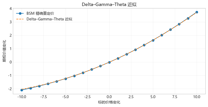

图 1.15 Black–Scholes 模型下期权价值的 Delta–Gamma–Theta 近似。

图 1.15 中，在本例一个交易日的时间间隔和 \(\pm10\%\) 的股价变动范围内，Delta–Gamma–Theta 估计与 BSM 精确重定价的曲线几乎重合。正的 Gamma 项在股价上涨和下跌情景中都加入正的二次修正，刻画了价格曲线向上弯曲的形状。当股价不变时，估计中的价格变化为 \(\Theta/250\)，对应一个交易日的时间价值损失。因此，本例只用初始点的三个 Greeks，就能准确近似图中各股价情景下的期权价值变化。

1.10 隐含波动率

在 Black Scholes 模型中，期权价格由以下因素决定：

• 标的资产当前价格 \(S_0\)；
• 标的资产波动率 \(\sigma\)；
• 期权行权价 \(K\)；
• 期权期限 \(T\)；
• 无风险利率 \(r\)。

其中 \(S_0,K,T,r\) 均为已知。所以只需知道波动率，就可推出期权价格。反之，知道期权价格，也可以推出波动率。我们在第 1.3.1 节已经介绍过波动率可以根据股票的历史价格来估计，这种方法得到的波动率称为历史波动率（historical volatility）。但若使用历史波动率对期权定价，得到的理论价格通常与期权的市场价格相差甚远。在实践中，通常会根据期权价格来反推出波动率。这种方法得到的波动率称为隐含波动率，它是用某个期权定价模型，从该期权的市场价格（权利金）中计算出的波动性，反映了市场对 未来标的资产波动率的预期。换言之，一个期权的隐含波动率在被代入定价模型后，所得出的理论价格将和该期权的市场价格相吻合，即

\[ \sigma_{\mathrm{imp}}: V(\sigma_{\mathrm{imp}},S_0,K,T,r)=V_{\mathrm{market}}. \]

由于期权 Vega \(>0\)，标的资产波动率越高，欧式期权价格也越高。图 1.16 显示，在 BSM 模型下欧式看涨期权价格确实是波动率 \(\sigma\) 的递增函数。当 \(S_0,K,T>0\)，且市场价格严格介于第 1.10.1 节给出的价格下界与上界之间时，存在唯一的有限正隐含波动率。

# 图 1.16：设置期权参数并计算不同波动率下的价格
iv_spot = 100.0
iv_strike = 120.0
iv_maturity = 1.0
iv_rate = 0.05
iv_cp = 1
iv_market_price = 2.0

volatility_values = np.linspace(0.01, 0.80, 250)
volatility_prices = np.array(
    [
        black_scholes_formula(
            volatility,
            iv_spot,
            iv_strike,
            iv_maturity,
            iv_rate,
            iv_cp,
        )
        for volatility in volatility_values
    ]
)

# 图 1.16：Black–Scholes 欧式看涨期权价值与波动率的关系，其中 $S_0=100$、$r=5\%$、$T=1$、$K=120$
fig, ax = plt.subplots(figsize=(8, 4.2))
ax.plot(volatility_values, volatility_prices)
ax.set_xlabel("波动率")
ax.set_ylabel("看涨期权价值")
ax.set_title("看涨期权价值与波动率")
ax.grid(True, alpha=0.25)
fig.tight_layout()
plt.show()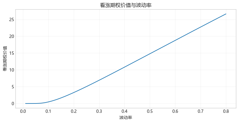

图 1.16 Black–Scholes 欧式看涨期权价值与波动率的关系，其中 \(S_0=100\)、\(r=5\%\)、\(T=1\)、\(K=120\)。

1.10.1 用数值解法求解隐含波动性

一般来说，隐含波动率需要用数值解法求解，比如可以使用二分法,见Python 程序 1.12。二分法只需要知道价格误差的符号，并把波动率区间不断对半切分。令

\[ f(\sigma)=V(\sigma,S_0,K,T,r)-V_{\mathrm{market}}. \]

对于无分红欧式看涨期权，市场价格必须满足

\[ \max(S_0-Ke^{-rT},0)\leq V_{\mathrm{market}}\leq S_0. \]

看跌期权相应满足

\[ \max(Ke^{-rT}-S_0,0)\leq P_{\mathrm{market}}\leq Ke^{-rT}. \]

在满足无套利边界的情况下，二分法的上下界必须使价格误差异号，即 \(f(\sigma_{\mathrm{low}})f(\sigma_{\mathrm{high}})\leq0\)。从一个足够宽的区间开始，每一轮取中点：如果中点对应的模型价格高于市场价格，就把上界移到中点；如果模型价格低于市场价格，就把下界移到中点。每轮迭代将区间宽度减半；经过 \(m\) 轮后，宽度为初始宽度的 \(2^{-m}\)，中点与区间内根的距离至多为该宽度的一半。

二分法过程示意图

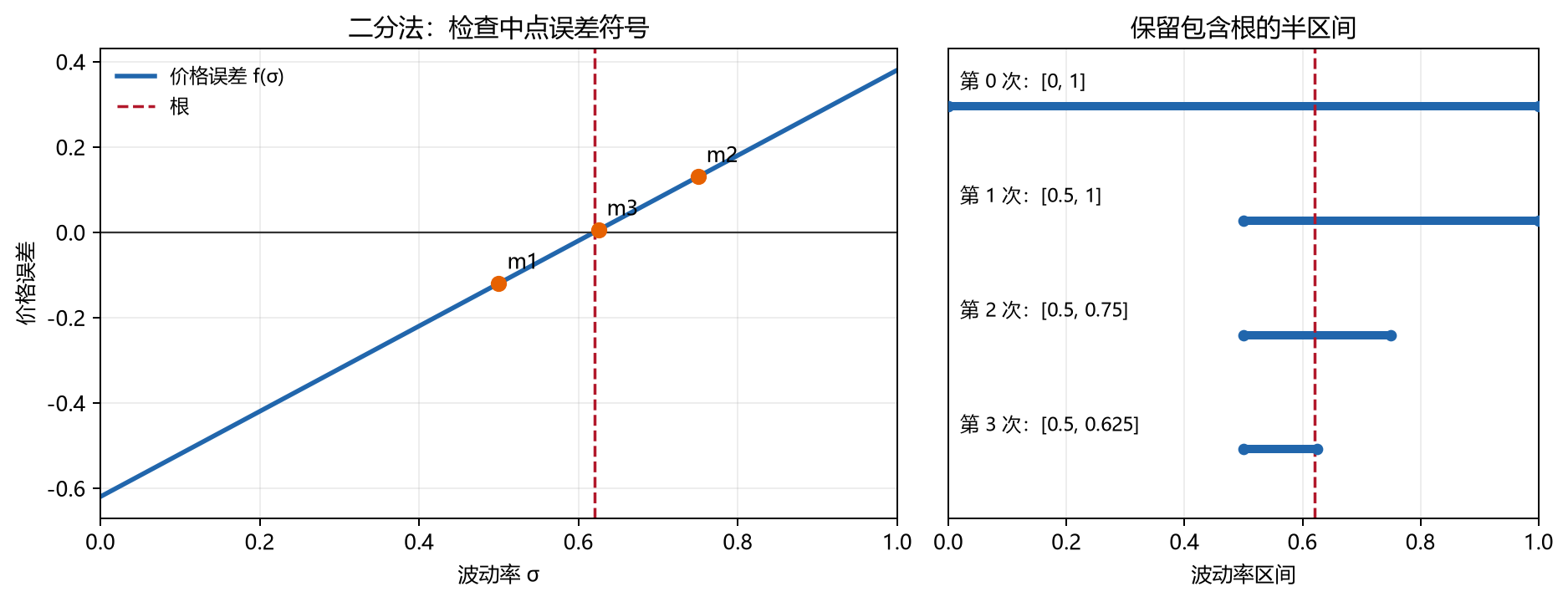
二分法过程示意图。 左图表示在价格误差函数上检查中点的符号；右图表示每次保留包含根的半区间，直到区间足够窄。

公式与代码对应

target 是市场期权价格，low 和 high 是波动率搜索区间的两个端点，mid 是区间中点。error 对应 \(f(\sigma)=V_{\rm BS}(\sigma)-V_{\rm market}\) 在中点的值，用它的符号选择下一轮的区间。

Python程序 1.12：二分法隐含波动率函数

def implied_volatility_bisection(
    target, S0, K, T, r, cp, low=1e-8, high=5.0
):
    if low <= 0 or high <= low:
        raise ValueError("波动率区间必须满足 0 < low < high")
    low_error = black_scholes_formula(low, S0, K, T, r, cp) - target
    high_error = black_scholes_formula(high, S0, K, T, r, cp) - target
    if low_error * high_error > 0:
        raise ValueError("市场价格不在给定波动率区间内")
    # 二分法返回隐含波动率和每轮迭代记录
    iteration_rows = []
    for iteration in range(100):
        mid = 0.5 * (low + high)
        error = black_scholes_formula(mid, S0, K, T, r, cp) - target
        iteration_rows.append(
            {
                "迭代次数": iteration,
                "波动率区间下界": low,
                "波动率区间上界": high,
                "中点": mid,
                "价格误差": error,
            }
        )
        if abs(error) < 1e-10:
            return mid, pd.DataFrame(iteration_rows)
        if error > 0:
            high = mid
        else:
            low = mid
    return 0.5 * (low + high), pd.DataFrame(iteration_rows)

# 程序 1.12 示例：求解隐含波动率并显示二分迭代
target_price = iv_market_price
bisection_volatility, bisection_iterations = implied_volatility_bisection(
    target_price,
    iv_spot,
    iv_strike,
    iv_maturity,
    iv_rate,
    iv_cp,
)
bisection_iterations.head(8)

	迭代次数	波动率区间下界	波动率区间上界	中点	价格误差
0	0	1.000000e-08	5.000000	2.500000	75.443706
1	1	1.000000e-08	2.500000	1.250000	41.285267
2	2	1.000000e-08	1.250000	0.625000	17.762321
3	3	1.000000e-08	0.625000	0.312500	5.383629
4	4	1.000000e-08	0.312500	0.156250	-0.157154
5	5	1.562500e-01	0.312500	0.234375	2.456042
6	6	1.562500e-01	0.234375	0.195313	1.088574
7	7	1.562500e-01	0.195313	0.175781	0.446166

二分法求解结果。 在本例中，二分法最终得到

\[ \sigma_{\mathrm{imp}}^{\mathrm{(bisect)}}\approx 0.161483, \]

即隐含波动率约为 \(16.15\%\)。将该波动率代入 BSM 看涨期权定价函数，得到的价格约为 \(2\)，与给定的市场价格一致。

1.10.2 Vega 与隐含波动率

因为 Black-Scholes 模型中期权价格对于波动率的一阶导数 \(\partial V/\partial\sigma\) 可以由解析式表达，所以可以使用 Newton 迭代法更有效率地找到隐含波动率。在第 1.9.6 节我们已经推出 \(\nu=\partial V/\partial\sigma\) 的解析式（1.9.23），可应用于隐含波动率的求解。这可以由 Python 程序 1.13 来实现。Newton 迭代为

\[ \sigma_{m+1}=\sigma_m-\frac{V(\sigma_m)-V_{\mathrm{market}}}{\operatorname{Vega}(\sigma_m)}. \]

Newton 法把价格误差 \(\delta V\) 除以 Vega，给出波动率调整 \(\delta\sigma=-\delta V/\operatorname{Vega}\)。例如，价格误差为 0.1、Vega 为 20 时，调整量为 \(-0.005\)；Vega 为 0.01 时，同样误差对应的调整量为 \(-10\)。程序要求更新后的波动率为正；二分法则把更新限制在含根的正波动率区间内。下面固定 \(S_0=100\)、\(K=120\)、\(T=1\)、\(r=5\%\)、\(V_{\mathrm{market}}=2\)，让两种方法从不同角度逼近同一个隐含波动率。二分法记录每轮的区间和价格误差，Newton 法记录每轮的波动率和价格误差。

Newton 法过程示意图

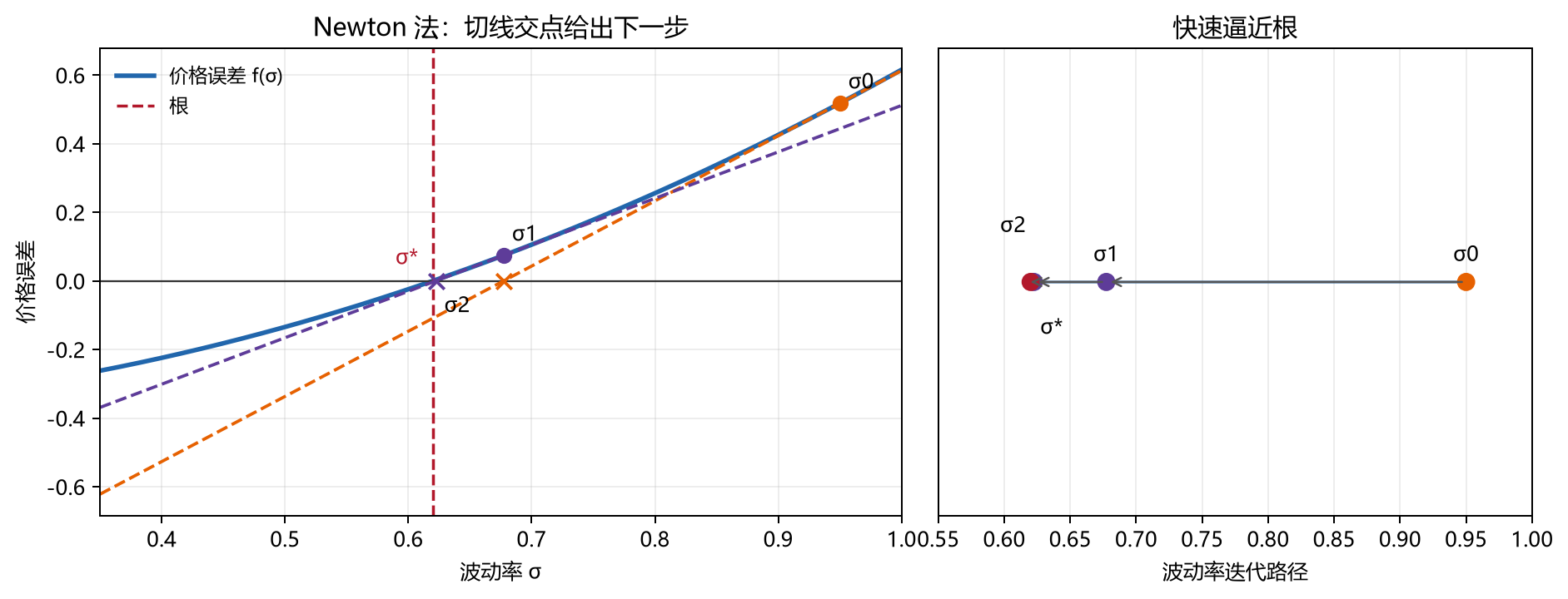
Newton 法过程示意图。 左图表示在当前点作切线，并把切线与横轴的交点作为下一次波动率；右图表示迭代点快速逼近根。

公式与代码对应

volatility 和 next_volatility 对应 \(\sigma_m\) 与 \(\sigma_{m+1}\)。error 对应 \(f(\sigma_m)\)，vega 对应 \(f\prime(\sigma_m)=\partial V_{\rm BS}/\partial\sigma\)，更新量为两者之比。

Python程序 1.13：Newton法隐含波动率函数

def implied_volatility_newton(
    target, S0, K, T, r, cp, initial=0.20, tolerance=1e-10, max_iterations=20
):
    '''Recover volatility by Newton iteration and return its trace.'''
    if initial <= 0:
        raise ValueError("初始波动率必须为正")
    volatility = initial
    iteration_rows = []
    for iteration in range(max_iterations):
        price = black_scholes_formula(volatility, S0, K, T, r, cp)
        d1 = (np.log(S0 / K) + (r + volatility**2 / 2) * T) / (
            volatility * np.sqrt(T)
        )
        vega = S0 * norm.pdf(d1) * np.sqrt(T)
        error = price - target
        iteration_rows.append(
            {"迭代次数": iteration, "波动率": volatility, "价格误差": error}
        )
        if abs(error) < tolerance:
            break
        if not np.isfinite(vega) or vega <= 0:
            raise ValueError("Vega 无效，无法继续 Newton 迭代")
        next_volatility = volatility - error / vega
        if not np.isfinite(next_volatility) or next_volatility <= 0:
            raise ValueError("Newton 步长得到非正波动率")
        volatility = next_volatility
    else:
        raise RuntimeError("Newton 法在指定迭代次数内未收敛")
    return volatility, pd.DataFrame(iteration_rows)

# 程序 1.13 示例：求解隐含波动率并显示 Newton 迭代
newton_volatility, newton_iterations = implied_volatility_newton(
    target_price,
    iv_spot,
    iv_strike,
    iv_maturity,
    iv_rate,
    iv_cp,
)
newton_iterations

	迭代次数	波动率	价格误差
0	0	0.200000	1.247477e+00
1	1	0.163389	5.811603e-02
2	2	0.161490	2.212975e-04
3	3	0.161483	3.319599e-09
4	4	0.161483	2.131628e-14

Newton 法求解结果。 从初始值 \(\sigma_0=0.20\) 出发，Newton 法最终得到

\[ \sigma_{\mathrm{imp}}^{\mathrm{(Newton)}}\approx 0.161483, \]

即隐含波动率约为 \(16.15\%\)。最后一轮的价格误差约为 \(2.1\times10^{-14}\)，与二分法得到的结果一致。

1.10.3 波动率曲面（Implied volatility surface）

BSM 模型使用固定波动率；市场期权反解得到的隐含波动率 \(\sigma_{\mathrm{imp}}(K,T)\) 则随行权价 \(K\) 和期限 \(T\) 变化。把隐含波动率作为行权价和期限的函数，就得到波动率曲面。图 1.17 给出了 2018 年 1 月 3 日 Euro Stoxx 50 在行权价 2,000 至 5,000、期限两周至十年范围内的隐含波动率。曲面的两个水平坐标分别对应行权价和到期时间，竖直坐标对应反解得到的隐含波动率。

2018年1月3日 Euro Stoxx 50 的隐含波动率曲面：行权价介于2,000至5,000，期限介于两周至十年。

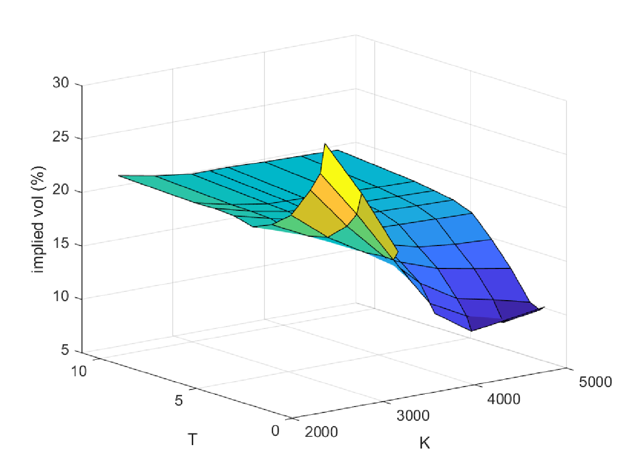
图 1.17 2018年1月3日 Euro Stoxx 50 的隐含波动率曲面：行权价介于 2,000 至 5,000，期限介于两周至十年。

1.10.4 波动率偏斜（Volatility skew）

从以上波动率曲面中选取期限为 2 年的期权，得到不同行权价对应的隐含波动率曲线，见图 1.18。可以看到行权价越高，隐含波动率越低，这种情况被称为 volatility skew（波动率偏斜）。由于波动率偏斜自从 1987 年的股灾以后才出现，有理论认为这是由于股票投资者担心股市崩盘，所以选择购买虚值看跌期权 (out-of-the-money put option) 来对冲股市风险，从而推高了低行权价看跌期权的价格（以及隐含波动率）。还有一种解释是购买实值看涨期权 (in-the-money call option) 相当于使用杠杆购买股票，这推高了对这类期权的需求，从而推高了低行权价看涨期权的价格（以及隐含波动率）。Bollen 和 Whaley（2004）发现，S&P 500 指数期权的隐含波动率变化与看跌期权的净买入压力有关

2018年1月3日 Euro Stoxx 50 两年期期权的隐含波动率与行权价。

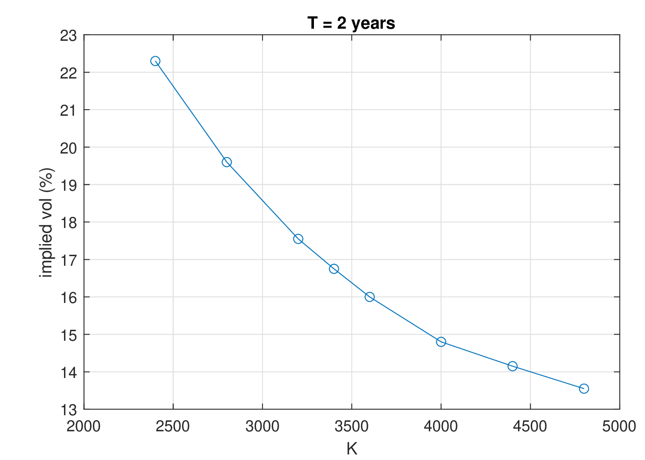
图 1.18 2018年1月3日 Euro Stoxx 50 两年期期权的隐含波动率与行权价。

参考文献

• Bachelier, L.（1900）. “Théorie de la spéculation.” Annales scientifiques de l’École Normale Supérieure, 第 3 系列, 17, 21–86. https://doi.org/10.24033/asens.476

• Samuelson, P. A.（1965）. “Rational Theory of Warrant Pricing.” Industrial Management Review, 6（2）, 13–32.

• Merton, R. C.（1976）. “Option Pricing When Underlying Stock Returns Are Discontinuous.” Journal of Financial Economics, 3, 125–144.

• Kou, S. G.（2002）. “A Jump Diffusion Model for Option Pricing.” Management Science, 48, 1086–1101.

• Beckers, S.（1981）. “A Note on Estimating the Parameters of the Diffusion-Jump Model of Stock Returns.” Journal of Financial and Quantitative Analysis, 16（1）, 127–140.

• Madan, D., Carr, P., & Chang, E.（1998）. “The Variance Gamma Process and Option Pricing.” European Finance Review, 2, 79–105.

• Figueroa-López, J. E., Lancette, S. R., Lee, K., & Mi, Y.（2011）. “Estimation of NIG and VG Models for High Frequency Financial Data.” In Handbook of Modeling High-Frequency Data in Finance, 1–25. John Wiley & Sons.

• Barndorff-Nielsen, O. E.（1997）. “Normal Inverse Gaussian Distributions and Stochastic Volatility Modelling.” Scandinavian Journal of Statistics, 24, 1–13.

• Schoutens, W.（2003）. Lévy Processes in Finance: Pricing Financial Derivatives. John Wiley & Sons.

• Cox, J., & Ross, S.（1976）. “The Valuation of Options for Alternative Stochastic Processes.” Journal of Financial Economics, 3, 145–166.

• Black, F., & Scholes, M.（1973）. “The Pricing of Options and Corporate Liabilities.” Journal of Political Economy, 81, 637–654.

• Aït-Sahalia, Y.（2004）. “Disentangling Diffusion from Jumps.” Journal of Financial Economics, 74, 487–528.

• Bollen, N. P. B., & Whaley, R. E.（2004）. “Does Net Buying Pressure Affect the Shape of Implied Volatility Functions?” The Journal of Finance, 59（2）, 711–753. https://doi.org/10.1111/j.1540-6261.2004.00647.x